Ekonomika ISSN 1392-1258 eISSN 2424-6166
2020, vol. 99(1), pp. 26–49 DOI: https://doi.org/10.15388/Ekon.2020.1.2
Effects of Energy Consumption on GDP: New Evidence of 24 Countries on Their Natural Resources and Production of Electricity
Rabnawaz Khan
School of Finance and Economics, Jiangsu University
People’s Republic of China
Email: khan.rab@stmail.ujs.edu.cn
YuSheng Kong
School of Finance and Economics, Jiangsu University
People’s Republic of China
Email: 1000001042@ujs.edu.cn
Abstract. Because of rapid economic expansion, China, the USA, and India have become the largest energy producers and sources of CO2 emissions in the world. They burned over 45% of global fuels in 2016. Meanwhile, the developing strategies of 24 polluted states to decrease fossil energy consumption without additional economic output. This paper explores the effect of world top polluted countries’ CO2 emission, their GDP and production of electricity by potential indicators and identifies the basic factors that contribute to changes in an environment where petroleum, natural gas, coal, nuclear, biomass, and other renewable energy and hydroelectric sources are examined with GDP per capita. We estimate our data for the period from 1968 to 2017 and use the GLM model. The results show that more production of electricity is causing abnormal CO2 emissions. The Granger causality test shows that there is a unidirectional relationship between energy consumption and economic advancement. Also, there is a short-run bidirectional causality that exists among the energy indicators. We find a unilateral causality between energy consumption and economic growth. Therefore, the consumption of energy might be conductive of 24 (polluted) countries and better economic development; the consumption of energy may be failsafe and guaranteed, while we should limit the resources of countries.
Keyword: CO2 emission; energy consumption; production of electricity; GDP
Received: 30/11/2019. Revised: 21/02/2020. Accepted: 02/03/2020
Copyright © 2020 Rabnawaz Khan, YuSheng Kong. Published by Vilnius University Press
This is an Open Access article distributed under the terms of the Creative Commons Attribution Licence, which permits unrestricted use, distribution, and reproduction in any medium, provided the original author and source are credited.
1. Introduction
Fossil fuels, like petroleum, natural gas, and coal, are estimated at 80% of energy consumption in the United States, and highest value recorded 101 quadrillion British thermal units (Btu) only in 2018, which was 81(Btu) of fossil fuel. Increases in natural gas consumption and petroleum drove the fossil fuel flow in 2018, while coal consumption fell by 4.3%. In 2005 in the USA, consumption peaked and since then declined by 42%. The onset of petroleum, coal, renewable energy, and nuclear power plants was a major energy indicator of energy consumption in the USA in the 18th to 21st centuries. We reached the natural gas consumption at a turning point with a value of 82.1 billion feet per day in 2018, and consumption has only increased by 37% in the last 8 to 10 years. In 2018, the petroleum product supplied reached 20.5 million barrels per day to 2005. Furthermore, the renewable energy consumption (hydroelectricity, wind, biomass, and solar energy) was 11.4% and it increased from the previous year.
China’s coal production has increased tenfold since 1960 and because of fossil-fuel CO2 emissions more than doubled alone in 2000. China’s emissions of CO2 have increased in the period of 1950 to 1997, and it became the world’s largest emitter of CO2 because of fossil-fuel. It recorded an annual 5.4% and growing with huge development. Almost half of the world’s cement had been produced in China; in 2008, it amounted to 1.38 billion metric tons. The per capita emission rate now stands at 1.34 metric tons of carbon (Boden, G.Marland, & R.J.Andres, 2011; Etemad, J.Luciani, P.Bairoch, & J.C.Toutian, 1991). China is the third largest natural gas consumption market and significantly relies on it for economic growth; among other primary energy sources, natural gas has been the optimal choice to resource energy transition, because it produces fewer CO2 emissions. The annual natural gas consumption was 16.26% in 2000 to 2007 with a 10.5% average annual economic growth (Fadiran, Adebusuyi, & Fadiran, 2019; Li, Cheng, & Gu, 2019). We recorded China’s natural gas consumption at 27.381 Cub ft/Day bn in 2018, and it increased in 1.17% from 2017. The petroleum consumption of coke (CO2, N2O and CH4) in China is exploding and had increased by 18.9% from 2010 to 2016. The petroleum related-CO2, N2O, and CH4 emissions reached 28, 143, and 870 million tonnes in 2016, respectively (Shan et al., 2018; X. Xu et al., 2018).
China’s renewable energy is comprised of hydroelectric, solar, wind, biofuel, biomass, and geothermal power. Pertaining to electricity, China is one of the leading country’s in form of renewable energy sources and who derive double its electricity from the USA. In 2013, the country had produced 378 GW of renewable power, from hydrochloric and wind power. Fig 1 signifies the energy difference between production and consumption in the period of 2010–2016. China, the USA, and India’s production of energy and consumption was developing faster than that of Russia, Saudi Arabia, and Australia. The renewable energy sector of China is growing faster than its fossil fuels and nuclear power energy sources. The largest rise of CO2 emissions grew by 3% in China since 2013. Hence, in 2013 to 2016, China’s CO2 emissions fell and shifted away from smokestack industries; also, renewable energy is a source of booming power generation, and policies are being implemented to tackle air pollution. China started another construction boom using its coal resources and increased its production by 4.5% in 2018 and by 3.3.% in 2017. With the world’s largest population and fastest growing economy, China is by far the world’s top country among the 25 highest CO2 emitters. China’s CO2 emission rates are growing because of its huge economic development. In 2017, the CO2 emissions from fossil fuel were 46.44% and 74.92% higher than those of the USA and India (See Table 1 for a comparative analysis).
Carbon dioxide emissions of India have increased from 7.1% to 10.1% in 2011 to 2014, which has been stemming from the burning of fossil fuel and cement manufacture. The overall growth of energy consumption will be higher for future industries and economic development in India. The non-conventional sources of energy have reduced the CO2 emissions by 11.8% (Gupta, Jain, & Bansal, 1995; Kumar & Sinha, 1995). The fourth largest country is Russia. We have declared the Russian Federation as contributing in CO2 emissions after India, and we record an overall 14% increase with 0.99 kg in 2010 ($GDP). We have declared that the Russian Federation has increased and will increase in the level of greenhouse (GHG) emissions by 20 to 30% in the period of 1990 to 2030 (Ketenci, 2018; Pao & Tsai, 2011).
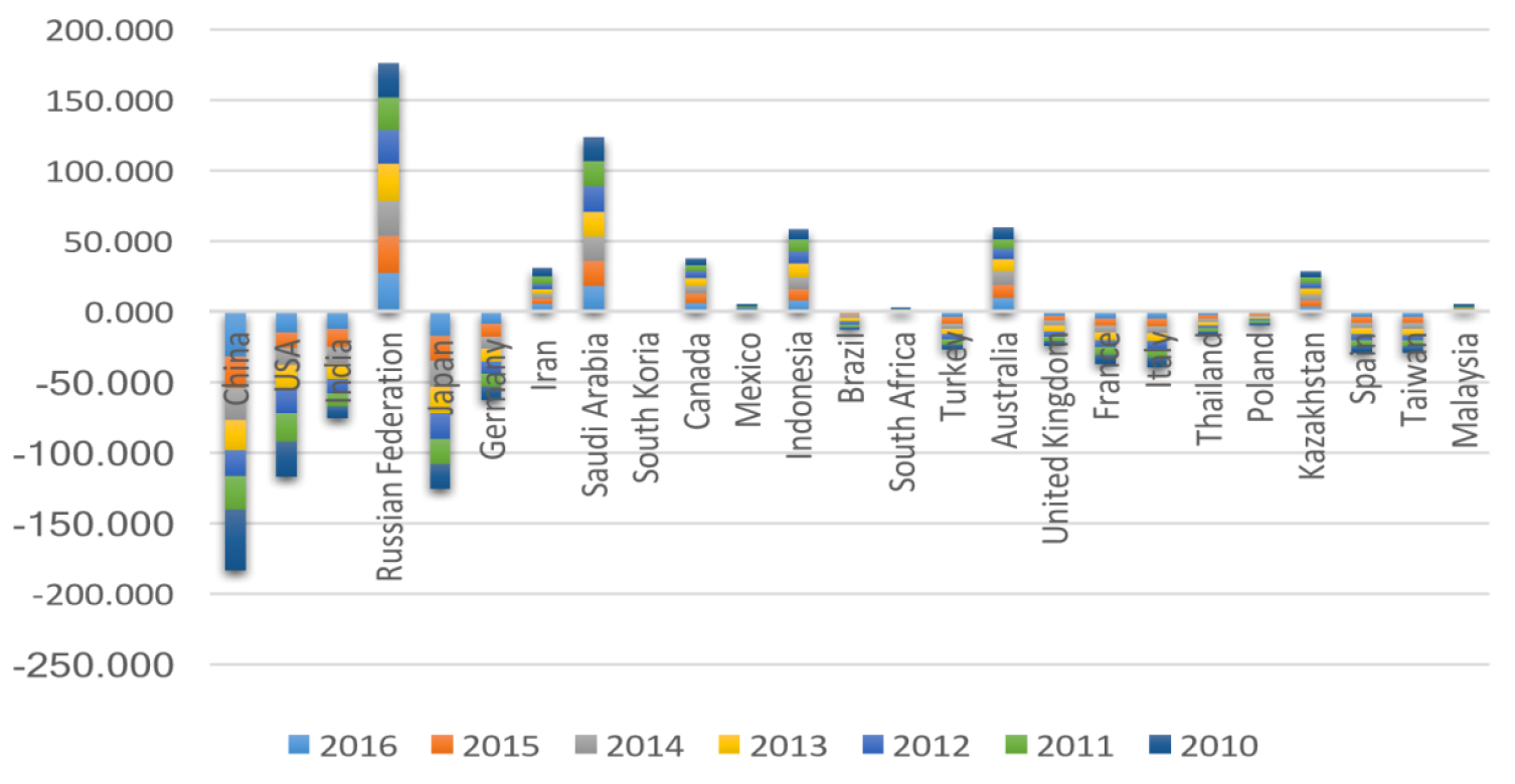
Fig. 1. Difference b/w energy production and consumption.
Source: US. Energy Information Admiration
The world’s 15 top countries are responsible for 72% CO2 emissions. According to the rankings of the CEOWORLD magazine, 25 countries were listed based on regional CO2 emissions from fossil fuel, methane emissions, CO2 emissions, and the changes were published in the 2018 Global Carbon Project (Table 1). We base this research paper on the rapid increase in CO2 emissions from petroleum, natural gas, coal, nuclear, biomas, other renewable energy and hydroelectric power, and its effects on the GDP of the top 24 polluted countries. Electricity production by natural resource results of carbon emissions in developing and developed countries. We can address this question through factors that cause the CO2 emission change and individual territory economic development and identify the force that changes the CO2 emission.
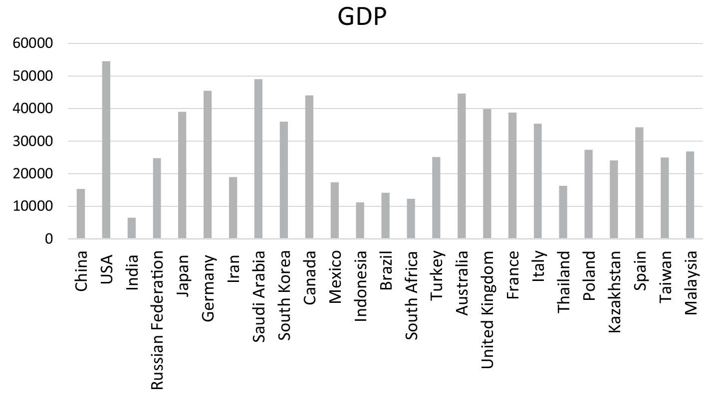
Fig. 2. GDP per capita 2017 ($)
The monetary terms of economic data, Gross Domestic Product (GDP) and per capita GDP, used in early studies to compare energy intensity were not examined in the top 24 countries of the high-ranking CO2 emissions and economic development. However, energy efficiency indicators were influenced by petroleum, natural gas, coal, nuclear, biomas, other renewable energy and hydroelectric with per capita of GDP, therefore leading to misleading efficiency conclusions. If, such as the economic growth of the 24 countries will increase, the energy use of the economic efficiency indicator will rise, although the energy use per unit output will not change.
Table 1. 25 highest CO2-emitting countries
|
Countries |
||
|
Canada |
Italy |
|
|
USA |
Mexico |
Thailand |
|
India |
Indonesia |
Poland |
|
Russian Federation |
Brazil |
Kazakhstan |
|
Japan |
South Africa |
Spain |
|
Germany |
Turkey |
Taiwan |
|
Iran |
Australia |
Malaysia |
|
Saudi Arabia |
United Kingdom |
|
|
South Korea |
France |
|
Sources: Author compiling by the World’s Top 25 countries CO2 Emission.
According to the environmental Kuznets’s Curve, rapid economic growth has an influence on the environment. Advanced technology can reduce the impact of CO2 emissions on economic growth. Developed and civilized people prefer to live in zones free of CO2 and protect nature from the harmful gasses with the help of modified technology and primary energy sources (Kong & Khan, 2019). If population and the poverty control by economic development policies, through its effect on rural and urban population for timber and fuel, lead to an increase in CO2, it will therefore cause air pollution. By doing so, we eliminate the possibility of a bias in study results (Baek, 2017).
This study used the GLM method to identify the basic factors that contribute to changes in an environment in the 24 top polluted countries. Eight indicators – petroleum, natural gas, coal, nuclear, biomass, other renewable energy and hydroelectric power – were examined with GDP per capita. We organize the rest of the paper as follows. Section 2 discusses the relevant literature; Section 3 presents the research methodology. Section 4 discusses the results, and Section 5 concludes the paper.
2. Literature review
In a recent study, the researchers examined the effects of CO2 emissions by oil, gas, and renewable energy of 79 different countries in the period of 1965–2017 but did not classify the contribution of the top 24 countries’ economic development and CO2 emission levels by petroleum, natural gas, coal, nuclear, biomas, other renewable energy and hydroelectric power. We investigate the changes in the primary energy production and consumption in the panel data of 24 countries. The World Bank database is a reliable source for CO2 emissions, and we used it in the current analysis. We have elaborated on the effect of the CO2 emissions by primary energy consumption under optimal thresholds without nuclear and coal emissions. Energy consumption classifies on the basis of income and emission levels (Valadkhani, Nguyen, & Bowden, 2019). The climate change policies have been examined, and the results showed that transport carbon emission increased in top 7 countries (Solaymani, 2019). With the EU-27 aggregated energy consumption with LMDI at 3 levels, the research showed the R&D and efficiency technologies are the main showing elements of low CO2 emissions (Fernández González et al. 2014. We analyze the BRICS countries results, the use of biomass in energy consumption for a sustainable environment, and showed an energy dependency along a rapid economic growth (Aydin, 2019). The 17 emerging countries were examined and the results showed the change in economic growth and renewable energy consumption with economic growth. The results show the conservation policies of energy do not have any adverse effect on the economic development of 16 countries; some strengths of the current analysis in earlier applications are as follows.
Table 2. Literature by different states
|
Countries |
Study |
Database |
Econometric techniques |
Periods |
Outcomes |
|
China |
(Kang, Islam, & Kumar Tiwari, 2019; B. Xu & Lin, 2019; G. Xu, Schwarz, & Yang, 2019) | International Energy Agency (IEA) | Non parametric regression model, NARX and VAR model. |
2000-2015 1965-2015 2017-2050 |
Natural gas consumption has effect in the eastern region. The coal consumption adds huge emissions. Impact of CO2 on GDP and a positive shock to CO2. |
|
USA |
(Chen, Shi, Shen, Huang, & Wu, 2019; Jiang, Wang, & Li, 2018) | World Input-Output Database (WIOD) | Geographical Detector Model | 1995-200 | 45% global CO2 emission produced from China and USA and production structure effect on environment. |
|
India |
(Anandarajah & Gambhir, 2014) | The Energy Resources Institute (TERI) | TIAM-UCL model | 2030-2050 | 34% energy consumption by renewable energy and 52% in 2050 |
|
Russian |
(C. Cheng, Ren, Wang, & Yan, 2019) | Organization for Economic Cooperation and Development (OECD) | OLS regression | 2000-2012 | GDP has created negative impacts on CO2 emission in EU-28 countries. |
|
Japan |
(Cai, Sam, & Chang, 2018) | World Development Indicators (WDI) | ARDL | 1965-2015 | As a dependent variable the integration exists in Japan |
|
Germany |
(González, Marrero, Rodríguez-López, & Marrero, 2019) | EU-13 | Dynamic panel data | 1990-2105 | CO2 emission have been given positive implementation to technological progress and changes. |
|
Iran |
(Hosseini, Saifoddin, Shirmohammadi, & Aslani, 2019) | WDI | multiple linear regression (MLR) | 1971-2014 | Iran include top CO2 emitted country and 30% increase in 2030. |
|
Saudi Arabia |
(Alkhathlan & Javid, 2015) | BP Statistical Review of World Energy | Structural Time Series Models (STSMs) | 1971-2013 | The CO2 emission grow by oil consumption |
|
South Korea |
(Jeong, Hong, & Kim, 2018) | MFHC Multi-family housing complex | Quartile |
CO2 emission reduction target by 2030 |
The results indicated CO2 emission benchmark for MFHCs can be applied. |
|
Canada |
(Cai et al., 2018) | WDI | ARDL | 1970-2015 | Canada use energy efficiency to reduce CO2 emission. |
Sources: Author literature review about the top ten CO2 emission countries.
3. Methodology
3.1. Generalized Linear Models (GLMs)
GLM model is used to analyze the extended linear regression to non-linear systematic and non-normal stochastic components (McCullagh, 1989). The GLM approach shows the response of the energy, natural gas, coal rent, nuclear energy, oil gas and coal, and renewable energy consumption in the six groups of carbon emissions. CO2 emission hypothesis, we followed the approach (K. Dong, Sun, & Dong, 2018; Kang et al., 2019; Ohashi et al., 2017). The relationship between GDP, energy, natural gas, coal rent, nuclear energy oil, gas, coal renewable energy consumption and total population Eq. 1 and GDPG Eq. 2.


Where GDP and GDPG shows the growth rate and growth rate per capita and i=1….,24 and t=1968…., 2017 divulge the country and time, where the GDP and GDPG effects, which we take from the CO2 emission from Energy, Natural Gas, Coal Rent, Nuclear Energy, Oil Gas and Coal, and Renewable energy consumption. αit shows country fixed effect and β1t – β14t are parameters for elasticities in Eq 1 and Eq 2, which are showing each explanatory variable of the panel ϵit, shows estimated residual further in each group of variables. The research intention based on causal link between Energy, Natural Gas, Coal Rent, Nuclear Energy, Oil Gas and Coal, and Renewable Energy Consumption with GDP and GDPG. The GLM yield sturdy and useful tool to estimate in a regression and estimated variables are not exogenous, autocorrelation and heteroscedasticity within exist. (Chong et al., 2019; Hosseini et al., 2019). We apply the GLM on an individual group to analyze the impact of the explanatory variable in each group on CO2 emission.
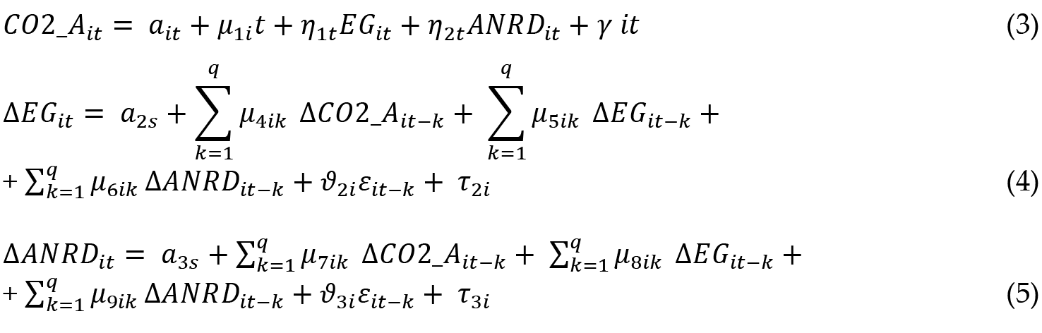
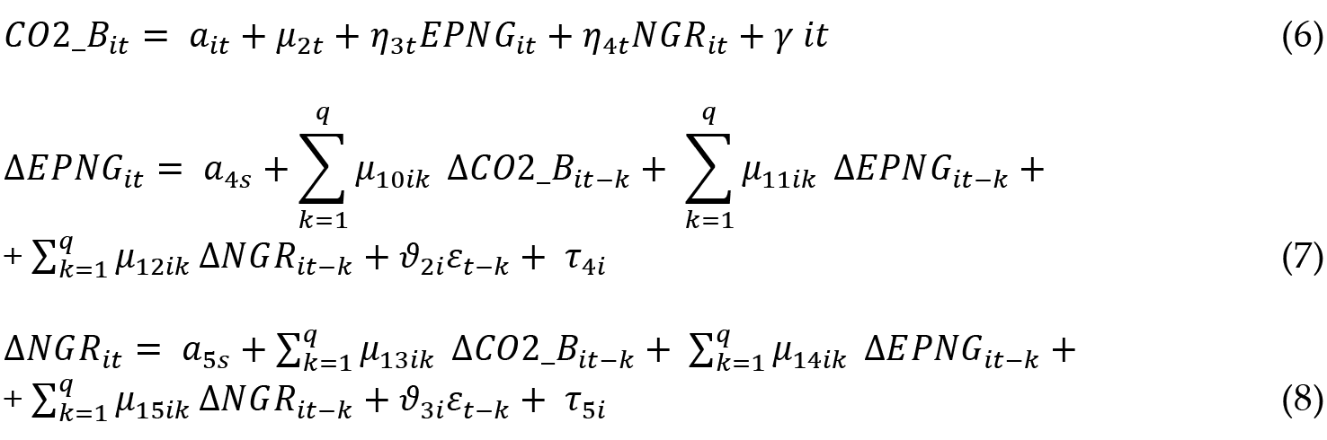
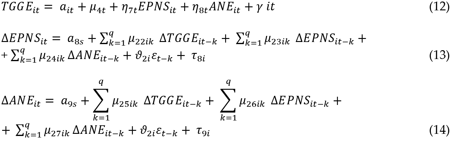
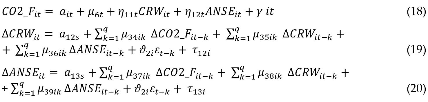
The Energy consumption was analyzed by energy use and natural resources Eq. 3-5. and cause of CO2 emission. Natural gas consumption was analyzed by the production of electricity and natural gas Eq. 6-8. and cause of CO2 emission. Coal rent consumption was analyzed by production of electricity and coal rents with causes of CO2 from solid fuel Eq. 9-11. Nuclear energy consumption was analyzed by production of electricity of nuclear resources and nuclear energy with causes of green gas emission Eq. 12-14. Oil gas and coal consumption was examined by electricity access and the production of electricity from oil gas and coal with causes of intensity of CO2 Eq. 15-17. Renewable energy consumption was analyzed by renewable and waste combustion and net saving includes emission damages with causes of CO2 from manufacturing industries Eq. 18-20.
Group A: Energy consumption
Group B: Natural gas consumption
Group C: Coal rent consumption
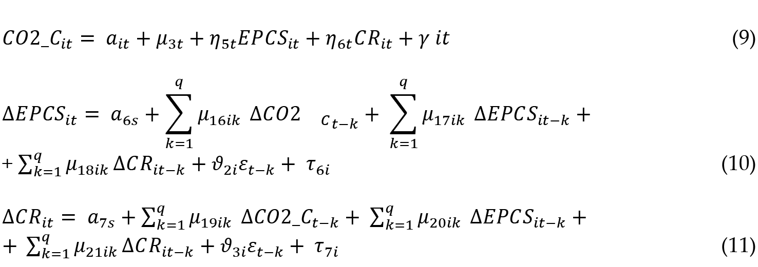
Group D: Nuclear energy consumption
Group E: Oil, Gas and Coal consumption

Group F: Renewable Energy consumption
All above six groups data of each country. In addition, we identify the parameter and ai and μt effect with a deterministic trend. All above six groups Granger with F-test among them. Where the first difference specifies by as ∆, lag of length showed by at q one conferring to likelihood ratio-test and show τ uncorrelated serial error term.
3.2. Data Description
This paper investigates the relationship among CO2 in six groups of individual variables. The economic growth and per-capita growth shows the dynamic relationship with CO2_A, CO2_B, CO2_C, TGGE, CO2_INT and CO2_F. The level of CO2 emission was and its effects on the GDP of the top 24 polluted countries with a huge production of electricity by different resources in the period of 1968–2017 were analyzed and selected as the research samples given in Table 3. The research variables were constructed as follows with the meaningful statistics tools in Table 4.
Table 3. Variables descriptions
|
Variables |
Symbol |
Description |
Data Source |
|
Natural resources |
ANRD |
Natural resource depletion and mineral depletion |
NY.ADJ.DRES.GN. ZS |
|
Energy use |
EG |
Primary energy before transformation |
EG.USE.PCAP.KG. OE |
|
Energy consumption |
CO2_A |
CO2 produced during consumption of solid, liquid and gas |
EN.ATM.CO2E.KT |
|
Natural gas |
NGR |
Natural gas rents and total costs of production |
NY.GDP.NGAS. RT. ZS |
|
Production of electricity from natural gas |
EPNG |
Electricity sources and natural gas |
EG.ELC.NGAS.ZS |
|
Natural gas consumption |
CO2_B |
CO2 emission from liquid fuel consumption |
EN.ATM.CO2E.GF. KT |
|
Coal rents |
CR |
Coal rent value and their costs of production. |
NY.GDP.COAL. RT. ZS EG.ELC.COAL. ZS |
|
Production of electricity from coal sources |
EPCS |
Sources of electricity used to generate electricity |
EG.ELC.COAL. ZS |
|
Carbon emission from solid fuel |
CO2_C |
CO2 emissions from consumption of solid fuel |
EN.ATM.CO2E.SF. KT |
|
Nuclear Energy |
ANE |
Non carbohydrate energy does not produce CO2, when generated |
EG.USE.COMM.CL. ZS |
|
Production of electricity from nuclear sources |
EPNS |
Electricity produced by nuclear power plants |
EG.ELC.NUCL. ZS |
|
Greenhouse gas emission |
TGGE |
CO2 excluding burning of short cycle biomass |
EN.ATM.GHGT. KT. CE |
|
Production of electricity from oil, gas, and coal sources |
EPOGC |
Oil, gas and liquids is source of electricity |
EG.ELC.FOSL. ZS |
|
Electricity access |
AE |
Electrification data collected from industries |
EG.ELC.ACCS. ZS |
|
Intensity of Carbon dioxide |
CO2_INT |
CO2 emission from use of coal as source of energy |
EN.ATM.CO2E.EG. ZS |
|
Net saving includes emission damages |
ANSE |
Natural savings and particular emissions damage. |
NY.ADJ.SVNG.GN. ZS |
|
Renewable and waste combustion |
CRW |
Combustible renewable as percentage of energy use |
EG.USE.CRNW. ZS |
|
Carbon emission from manufacturing industries |
CO2_F |
CO2 emissions from combustion of fuels industry |
EN.CO2.MANF. ZS |
|
Total population |
PT |
De facto population |
SP.POP.TOTL |
|
Growth of domestic product |
GDP |
Annual percentage growth on local currency |
NY.GDP.MKTP.KD. ZG |
|
Per-capita growth (GDP) |
GDPG |
Annual percentage growth rate of GDP |
NY.GDP.PCAP.KD. ZG |
Sources: Selection based on accessibility of database of World Bank. Variable’s definition indicated in Table 3.
Table 4. Descriptive statistics
|
Descriptive analysis |
Mean |
Median |
Std. Dev. |
Observations |
|
|
Energy consumption |
ANRD |
2.848 |
1.236 |
4.516 |
1030 |
|
EG |
2848.151 |
2512.106 |
2080.778 |
1059 |
|
|
CO2_A |
754203.900 |
346876.200 |
1336399.000 |
1021 |
|
|
Natural gas consumption |
NGR |
0.370 |
0.068 |
0.771 |
1032 |
|
EPNG |
16.525 |
8.180 |
20.226 |
1071 |
|
|
CO2_B |
121734.000 |
46985.270 |
248984.800 |
1021 |
|
|
Coal rent consumption |
CR |
0.411 |
0.048 |
0.901 |
1028 |
|
EPCS |
35.664 |
27.698 |
30.069 |
1071 |
|
|
CO2_C |
308747.000 |
72293.070 |
768653.000 |
1044 |
|
|
Nuclear energy consumption |
ANE |
6.312 |
2.941 |
8.429 |
1058 |
|
EPNS |
8.005 |
0.316 |
14.958 |
1059 |
|
|
TGGE |
1160331.000 |
550135.800 |
1649953.000 |
997 |
|
|
Oil, Gas and Coal consumption |
EPOGC |
68.787 |
75.064 |
24.639 |
1071 |
|
AE |
95.263 |
100.000 |
12.024 |
559 |
|
|
CO2_INT |
2.703 |
2.623 |
0.955 |
993 |
|
|
Renewable energy consumption |
ANSE |
9.260 |
8.738 |
7.136 |
600 |
|
CRW |
9.802 |
3.880 |
14.474 |
1059 |
|
|
CO2_F |
23.270 |
21.289 |
11.517 |
1047 |
|
|
GDP effects |
PT |
153000000.000 |
57000451.000 |
281000000.000 |
1195 |
|
GDP |
3.846 |
3.707 |
4.809 |
1075 |
|
|
GDPG |
2.483 |
2.544 |
4.602 |
1075 |
|
Sources: Calculated by the authors. Variable’s definition indicated in Table 3.
4. Empirical estimation results and discussions
Table 4 shows the Energy, Natural Gas, Coal rent, Nuclear Energy Oil, Gas and Coal Renewable Energy consumption, variables mean in the period of 1968–2017, and countries analyzed by the CO2 emission. In each group, CO2_A, CO2_B, CO2_C, TGGE, CO2_INT and CO2_F have tested on an individual basis with explanatory variables. We applied the descriptive statistics tests to judge whether the explanatory variable works with response to the variables. The China (CO2_C), USA (CO2_A, CO2_B, TGGE), Saudi Arabia (CO2_INT) and Korea (CO2_F) register the highest mean, while Korea, Malaysia, Indonesia (CO2_A, CO_B), the Iran Islamic Republic, Malaysia, Mexico (CO2_C, TGGE), Indonesia, Brazil, and the Russian Federation (CO2_F) register the lowest mean. The highest mean value concludes that all predictors with CO2_A, CO2_B, CO2_C, TGGE, and CO_F integrated countries of economic development (Fig 3). The results were computed by a Generalized Linear Model (GLM) and, to remove any inconvenience, considered using a stationary test by a 1st generation unit root test and individual intercept in level. Most of the statistics test rejects the null hypothesis, including the variables stationary at the level in individual groups.
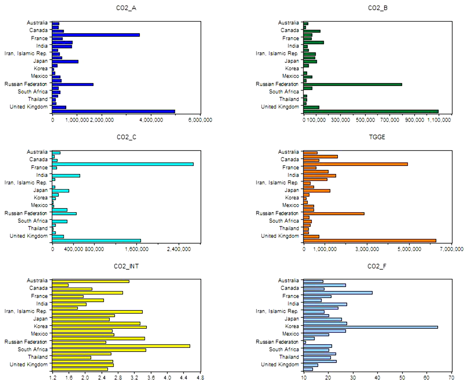
Fig. 3. Countries distribution by mean
4.1. Unit root and co-integration
Before analysis, the unit root test applied so ADF, PP, LLC, IPS and BR whether the variables in group A (ANRD, EG, CO2_A), group B (NGR, EPNG, CO2_B), group C (CR, EPCS, CO2_C), group D (ANE, EPNS, TGGE), group E (EPOGC, AE, CO2_INT), group F (ANSE, CRW, CO2_F) and group G (PT, GDP, GDPG) have unit-root or not. The test results rejected the null hypothesis and concluded that the selected variables are not stationary, whether the cointegration exists among the variables. In the 1st stage, VAR was estimated and the model proved to stable as shown in Table 5.
Table 5. Estimation by VAR
|
Group A [t-test] |
ANRD (-1) |
ANRD (-2) |
EG (-1) |
EG (-2) |
CO2_A (-1) |
CO2_A (-2) |
|
ANRD |
0.841[25.502] |
0.072[2.206] |
0.000[-0.032] |
0.000[-0.003] |
0.000[0.796] |
0.000[-0.821] |
|
EG |
3.676[1.525] |
3.525[1.470] |
1.028[27.910] |
-0.028[-0.763] |
0.000[2.291] |
0.000[-2.311] |
|
CO2_A |
(755.402) [-0.767] |
1446.458[1.475] |
(81.432) [-5.407] |
77.684[5.110] |
1.700[58.061] |
(0.692) [-22.764] |
|
Group B [t-test] |
NGR (-1) |
NGR (-2) |
EPNG (-1) |
EPNG (-2) |
CO2_B (-1) |
CO2_B (-2) |
|
NGR |
1.029[30.557] |
(0.128) [-3.739] |
(0.002) [-0.660] |
0.004[1.312] |
0.000[2.103] |
0.000[-2.019] |
|
EPNG |
0.317[0.852] |
(0.406) [-1.073] |
1.150[33.597] |
(0.154) [-4.444] |
0.000[-0.010] |
0.000[-0.032] |
|
CO2_B |
(2363.177) [-1.640] |
2431.678[1.664] |
176.159[1.331] |
(157.399) [-1.174] |
1.133[32.576] |
(0.129) [-3.695] |
|
Group C [t-test] |
CR (-1) |
CR (-2) |
EPCS (-1) |
EPCS (-2) |
CO2_C (-1) |
CO2_C (-2) |
|
CR |
0.670[20.059] |
0.142[4.279] |
(0.001) [-0.217] |
0.005[0.774] |
0.000[0.964] |
0.000[-0.979] |
|
EPCS |
0.039[0.211] |
0.261[1.437] |
0.990[29.446] |
(0.004) [-0.105] |
0.000[0.093] |
0.000[-0.091] |
|
CO2_C |
(2224.419) [-0.828] |
3786.855[1.421] |
(1644.893) [-3.335] |
1645.273[3.355] |
1.676[58.142] |
(0.666) [-21.959] |
|
Group D [t-test] |
ANE (-1) |
ANE (-2) |
EPNS (-1) |
EPNS (-2) |
TGGE (-1) |
TGGE (-2) |
|
ANE |
0.977[17.483] |
0.016[0.276] |
0.164[5.353] |
(0.155) [-5.043] |
0.000[0.400] |
0.000[-0.332] |
|
EPNS |
0.087[0.871] |
(0.099) [-0.980] |
1.284[23.492] |
(0.277) [-5.032] |
0.000[-0.071] |
0.000[0.106] |
|
TGGE |
(19665.7) [-1.065] |
22779.000[1.226] |
8362.019[0.828] |
(10844.630) [-1.066] |
0.696[21.843] |
0.333[10.166] |
|
Group E [t-test] |
EPOGC (-1) |
EPOGC (-2) |
AE (-1) |
AE (-2) |
CO2_INT (-1) |
CO2_INT (-2) |
|
EPOGC |
0.924[17.984] |
0.077[1.483] |
(0.054) [-0.725] |
0.050[0.702] |
1.602[1.263] |
(1.967) [-1.553] |
|
AE |
0.036[1.478] |
(0.023) [-0.963] |
0.529[15.075] |
0.404[12.162] |
0.112[0.187] |
(0.716) [-1.207] |
|
CO2_INT |
(0.001) [-0.565] |
0.002[0.795] |
(0.003) [-1.097] |
0.003[0.961] |
0.866[17.336] |
0.096[1.934] |
|
Group F [t-test] |
ANSE (-1) |
ANSE (-2) |
CRW (-1) |
CRW (-2) |
CO_F (-1) |
CO_F (-2) |
|
ANSE |
0.840[18.716] |
0.027[0.631] |
(0.394) [-1.751] |
0.378[1.716] |
0.116[1.785] |
(0.048) [-0.754] |
|
CRW |
0.006[0.747] |
(0.014) [-1.678] |
1.160[25.769] |
(0.179) [-4.068] |
(0.022) [-1.741] |
0.012[0.975] |
|
CO_F |
(0.026) [-0.877] |
0.031[1.067] |
(0.131) [-0.859] |
0.142[0.948] |
0.764[17.195] |
0.199[4.554] |
Sources: Calculated by the authors . Variable’s definition indicated in Table 3. VAR estimation were estimated with individual group restrictions and provide first lag coefficients of each group with t-test.
4.2. Pair wise Granger causality test
We applied a Granger causality test to confirm whether endogenous variables were treated as exogenous in individual groups. Ahead, selected variables co-integrated, we assessed to perform the Granger Causality Test (GCT) among variables as presented in Table 6. We accept the null hypothesis that CO2_A does not granger cause EG and ANRD and EG does not granger cause of ANRD and vice versa found in Energy consumption. In the Natural Gas, Coal rent, Nuclear Energy Oil, Gas and Coal Renewable Energy consumption, CO2_B, CO2_C, TGGE, CO2_INT and CO2_F does not granger cause of EPNG, EPCS, TGGE, EPOGC and CRW. (Emirmahmutoglu & Kose, 2011; Hao, Wang, Zhu, & Ye, 2018; Pao & Tsai, 2011). The Padroni Co-integration modified by Weighted Level Table 7. All the six group variables tested by co-integration methods rejected the null hypothesis and there is no co-integration relationship among variables. Table 8 (Kao C, 1995; P., 2004).
Table 6. Pairwise Granger Causality Test
|
Consumption |
Null Hypothesis |
F-Statistics |
|
Energy |
EG does not Granger Cause CO2_A |
22.529*** |
|
CO2_A does not Granger Cause EG |
2.026* |
|
|
ANRD does not Granger Cause CO2_A |
0.695* |
|
|
CO2_A does not Granger Cause ANRD |
1.098* |
|
|
ANRD does not Granger Cause EG |
25.303*** |
|
|
EG does not Granger Cause ANRD |
0.899* |
|
|
Natural gas |
EPNG does not Granger Cause CO2_B |
1.486* |
|
CO2_B does not Granger Cause EPNG |
0.576* |
|
|
NGR does not Granger Cause CO2_B |
1.478* |
|
|
CO2_B does not Granger Cause NGR |
4.00*** |
|
|
NGR does not Granger Cause EPNG |
0.820* |
|
|
EPNG does not Granger Cause NGR |
8.860*** |
|
|
Coal rent |
EPCS does not Granger Cause CO2_C |
5.198*** |
|
CO2_C does not Granger Cause EPCS |
0.101* |
|
|
CR does not Granger Cause CO2_C |
1.214* |
|
|
CO2_C does not Granger Cause CR |
0.508* |
|
|
CR does not Granger Cause EPCS |
3.583*** |
|
|
EPCS does not Granger Cause CR |
12.524*** |
|
|
Nuclear energy |
EPNS does not Granger Cause TGGE |
1.516* |
|
TGGE does not Granger Cause EPNS |
0.059* |
|
|
ANE does not Granger Cause TGGE |
0.94* |
|
|
TGGE does not Granger Cause ANE |
0.280* |
|
|
ANE does not Granger Cause EPNS |
0.392* |
|
|
EPNS does not Granger Cause ANE |
16.941*** |
|
|
Oil, Gas and Coal |
AE does not Granger Cause CO2_INT |
1.031*** |
|
CO2_INT does not Granger Cause AE |
1.802* |
|
|
EPOGC does not Granger Cause CO2_INT |
14.266*** |
|
|
CO2_INT does not Granger Cause EPOGC |
0.648* |
|
|
EPOGC does not Granger Cause AE |
2.659** |
|
|
AE does not Granger Cause EPOGC |
0.161* |
|
|
Renewable Energy |
CRW does not Granger Cause CO2_F |
2.492* |
|
CO2_F does not Granger Cause CRW |
0.756* |
|
|
ANSE does not Granger Cause CO2_F |
0.655* |
|
|
CO2_F does not Granger Cause ANSE |
7.376*** |
|
|
ANSE does not Granger Cause CRW |
7.148*** |
|
|
CRW does not Granger Cause ANSE |
3.148*** |
Sources: Calculated by the authors. Variable’s definition indicated in Table 3 ***,**, * indicates significance levels at 1%, 5% and 10%.
Table 7. Padroni Residual Co-Integration Modified table by Weighted level
|
Consumption |
Dimensions |
Panel |
Panel |
Panel |
Panel |
|
Energy |
Within |
5.283*** |
(1.833)*** |
(4.157)*** |
(1.744)*** |
|
Between |
|
0.224** |
(3.088)*** |
(1.595)*** |
|
|
Natural gas |
Within |
1.749** |
1.711** |
1.199** |
2.562** |
|
Between |
|
1.262** |
(0.851)** |
1.103** |
|
|
Coal rent |
Within |
(0.291)** |
2.488** |
(0.433)** |
2.41** |
|
Between |
|
0.373** |
(2.122)*** |
(0.148)** |
|
|
Nuclear energy |
Within |
5.562*** |
(1.261)** |
(4.168)*** |
(2.712)*** |
|
Between |
|
0.028** |
(4.701)*** |
(1.761)*** |
|
|
Oil, Gas and Coal |
Within |
(1.705)** |
0.192** |
(2.803)*** |
(4.354)*** |
|
Between |
|
1.027** |
(2.716)*** |
(1.284)*** |
|
|
Renewable energy |
Within |
(2.366)** |
1.191** |
(3.486)*** |
(0.250)** |
|
Between |
|
1.329** |
(4.620)*** |
(1.905)*** |
Note: Variable’s definition indicated in Table 3, *** specifies the significance levels at 1%, ** specifies the significance levels at 5%, * specifies the significance levels, at 1%, 5% and 10%.
Sources: Calculated by the authors.
Table 8. Covariance of GLM by GDPG
|
Variables |
GDPG |
CO2_A |
CO2_B |
CO2_C |
TGGE |
CO2_INT |
|
GDPG |
|
(2.238)*** |
(0.436)*** |
2.277*** |
2.435*** |
2.953*** |
|
CO2_A |
(2.239)*** |
|
32.626*** |
36.245*** |
11.833*** |
2.681*** |
|
CO2_B |
(0.437)** |
32.620*** |
|
(46.465)*** |
6.660*** |
1.295** |
|
CO2_C |
2.277*** |
36.245*** |
(46.465)*** |
|
7.438*** |
3.591*** |
|
TGGE |
2.243*** |
11.833*** |
6.660*** |
7.438*** |
|
(9.354)*** |
|
CO2_INT |
2.954*** |
11.833*** |
1.295** |
3.591*** |
(9.354)*** |
|
|
CO2_F |
1.604** |
2.681*** |
(10.871)*** |
(2.592)*** |
7.546*** |
(0.529)*** |
Note: Variable’s definition indicated in Table 3 ***, **, *, at 1%, 5% and 10%.
Sources: Calculated by the authors.
Although an excessive number of researchers examine the relationship of energy consumption with economic growth, very few do so on the group consumptions. No agreement has been reached on China’s energy consumption between economic development. Furthermore, the USA and India are also listed among the highest levels of energy consumption. Changes in economic growth and CO2 emissions have been examined in six-different comparisons. In contrast, the literature examined a unidirectional causality running from output to Energy, Natural Gas, Coal rent, Nuclear Energy Oil, Gas and Coal Renewable Energy consumption (Z. Cheng et al., 2017; Herrerias, Joyeux, & Girardin, 2013; Liang, Chai, Zhang, & Zhang, 2019; Lin, Fridley, Lu, Price, & Zhou, 2018; McGee & Greiner, 2019; Wolde-Rufael & Menyah, 2010). We should also note that in many countries except China the bulk of natural resources are still used, including Natural gas, Coal rent, Nuclear energy and renewable energy in a different group consumption.
The offered literature has already confirmed that the use of coal rent, natural gas, nuclear energy and renewable energy would impede economic development (F. Dong, Wang, Su, Hua, & Zhang, 2019; Jin & Kim, 2018). Natural gas to electricity causality and vice versa (Uribe, Guillen, & Mosquera-López, 2018). USA and China play an important role in the production of electricity from Coal and is a crucial factor for economic growth (Morales Pedraza, 2019; Wang et al., 2019). The USA provided substantial electricity by nuclear power and a meaningful increase in its capacity of production (Karney, 2019). The production of electricity from different fuel sources (oil, coal, and water) and prices of coal and oil are similar, it was found in the long run (Kharbach & Chfadi, 2018).
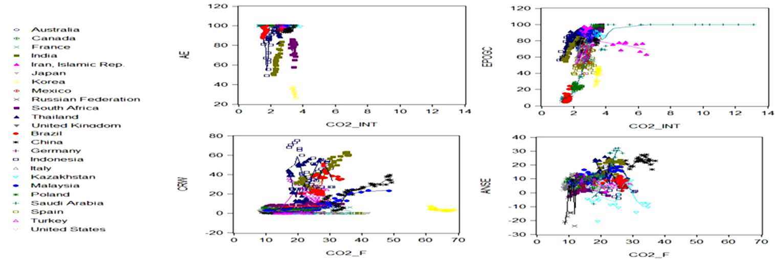
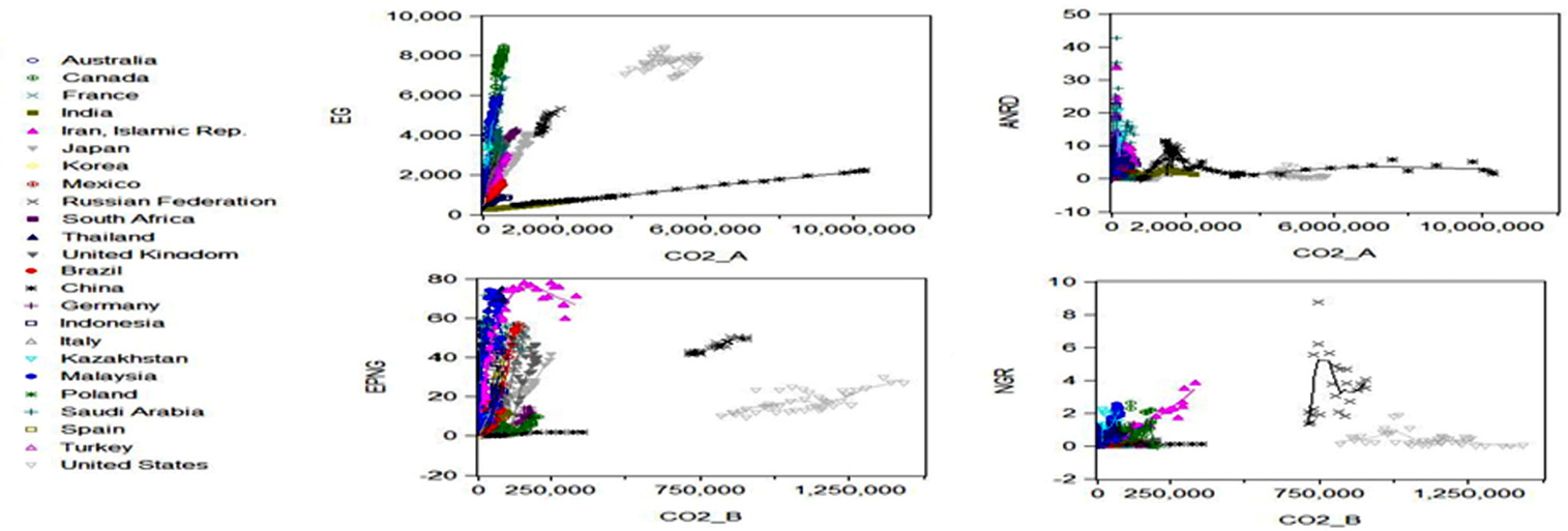
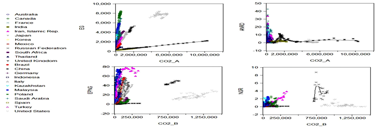
Group A & B
Group C & D
Group E & F
Fig. 4. Groups distribution by indicators
The results of estimation may be the reason for Granger causality for natural gas, coal rent, nuclear energy oil, gas and coal renewable energy consumption. The conclusion that ANRD, EG, NGR, EPNG, CR, EPCS, ANE, EPNS, EPOGC, AE, ANSE and CRW are not a Granger cause of CO2_A, CO2_B, CO2_C, TGGE, CO2_INT and CO2_F differs from the earlier study, some prior research using a mass of macro data, as most of earlier research found a positive effect on ANRD, CR, EPCS and ANSE on CO2_A, CO2_B, CO2_C (Acheampong, 2018; Mezghani & Ben Haddad, 2017). However, one reason for disparity may be that this study emphases the 25 polluted countries except Taiwan, while most of the previous studies have already discussed the environmental causes of GDP, but this study determined the six different groups of emission and individual effect of each variable with CO2_A, CO2_B, CO2_C, TGGE, CO2_INT and CO2_F. (Fig 4)
The Granger causality existence from energy consumption to ANRD, EG, NGR, EPNG, CR, EPCS, ANE, EPNS, EPOGC, AE, ANSE and CRW specifies the level of growth. Energy consumption precedes to increase of ANRD, EG, NGR, EPNG, CR, EPCS, ANE, EPNS, EPOGC, AE, ANSE and CRW in 24 top polluted countries, which can be assumes to be a feature of each individual country’s economic growth. There is some caution that the co-existent casualty in the coherent might not occur though the calculated results – this suggests the Granger causality. It shows test results significant causality among the variables. Almost a uni-directional causality could run from energy consumption and its effected-on GDP. In fact, however, if CO2_A, CO2_B, CO2_C, TGGE, CO2_INT and CO2_F is mismanaged into barren economic sectors, then the economic growth of an individual state is insignificant or cannot occur at all and may create big problems for nations.
4.3. Particular analysis by GLM
After computing the Granger causality among the variables, specifying the relationship and that needed by the Generalized Linear Model (GLM), it was seen that linear regression permits non-linear systematic components with non-normal stochastics in each group of energy consumption (Hardin, 2007; McCullagh, 1989). We get the conclusions of covariance of GLM by GDP. We estimate the covariance of reliant variables with GDPG in Ordinary and Huber-White.
We can observe that CO2_A, CO2_B, CO2_C, TGGE, CO2_INT and CO2_F affect GDPG at the significant level of 1% in the long term and that the 1% increase in energy consumption CO2_A, will cause of a GDPG increase with a 2.238. A 1% increase in CO2_B, CO2_C, TGGE, CO2_INT and CO2_F will cause a 0.436, 2.277, 2.435 and 2.953 increase in GDPG. The impact of CO2_A, CO2_B, CO2_C, TGGE, CO2_INT, CO2_F and GDPG is also positive at a significant level of 1%, and that a 1% rise is related to an increase in the GDPG results Table 8. We state the individual state consumption in Fig 5. The group covariance computed with Wald test. The impact of CO2_A, TGGE and CO2_INT is showing negative significant level of 1% in ANRD, ANE and AE with 11.248, 3.145 and 0.913 Wald test Table 9.
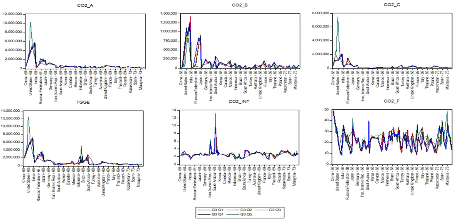
Fig. 5. Consumption level by individual state
Table 9. Stepwise regression
|
Consumption |
Variables |
Periods |
Wald-test |
||||
|
1st |
2nd |
3rd |
4th |
5th |
|||
|
1968-1977 |
1978-1987 |
1988-1997 |
1998-2007 |
2008-2017 |
|||
|
Energy |
ANRD |
4.800*** |
(0.379)** |
3.655*** |
8.222*** |
4.744*** |
2.831*** |
|
EG |
3.332*** |
(0.631)** |
(0.628)** |
0.610** |
(2.124)*** |
(2.253) *** |
|
|
CO2_A |
(0.933)** |
2.997*** |
3.161*** |
6.277*** |
6.318*** |
11.248*** |
|
|
Natural gas |
NGR |
0.502** |
1.789** |
(2.631)*** |
4.360*** |
0.784** |
7.804*** |
|
EPNG |
3.059*** |
(2.936)*** |
6.181*** |
2.858*** |
1.367** |
9.984*** |
|
|
CO2_B |
(0.918)** |
1.144** |
(0.256)** |
1.557** |
0.848** |
1.228** |
|
|
Coal rent |
CR |
(1.347)** |
(0.376)** |
(5.083)** |
1.886** |
0.434** |
0.554** |
|
EPCS |
2.802*** |
1.701*** |
5.996*** |
5.834*** |
3.358*** |
3.125*** |
|
|
CO2_C |
0.837** |
2.919*** |
2.575*** |
3.947*** |
4.274** |
7.795*** |
|
|
Nuclear |
ANE |
4.394*** |
1.118** |
1.322** |
1.842** |
0.946** |
16.684*** |
|
EPNS |
(0.906)** |
(0.360)** |
(0.848)** |
(1.345)** |
(1.325)** |
(2.535)*** |
|
|
TGGE |
1.783** |
3.463*** |
4.092*** |
8.350*** |
5.601*** |
3.145*** |
|
|
Oil, Gas and Coal |
EPOGC |
- |
- |
0.411** |
(1.883)** |
(1.444)** |
11.681*** |
|
AE |
- |
- |
(1.126)** |
(2.845)*** |
(3.019)*** |
24.442*** |
|
|
CO2_INT |
- |
- |
0.986** |
4.862*** |
3.485*** |
(0.913)** |
|
|
Renewable energy |
ANSE |
- |
- |
6.378*** |
(0.122)** |
3.568*** |
36.042*** |
|
CRW |
- |
- |
0.496** |
(1.436)** |
1.359** |
8.198*** |
|
|
CO2_F |
- |
- |
1.109** |
7.257*** |
0.974** |
10.542*** |
|
Note: Variable’s definition indicated in Table 3, ***, **, *, represent significance level at 1%, 5% and 10%.
Sources: Calculated by the authors.
4.4. Additional analysis
The above analysis implies the influence of each group and uses it on the other variables. The result does not specify the 10 years’ period of Energy, Natural gas, Coal rent, Nuclear energy, Oil and gas and Coal, and Renewable energy consumption. The stepwise regression shows five periods and each consists of 10 years’ duration.
Energy consumption of the 1st period shows negative at a significant level of 1% and uses that 1% increase CO2_A to decrease 1% in ANRD and EG. The Natural gas consumption 1st and 3rd periods are negative at a significant level and denote a 1% increase in CO2_B related to the decrease of NGR and EPNG. However, the 4th and 5th period positive at the significant level of 1% that a 1% rise in CO2_A, CO2_B, CO2_C, TGGE, CO2_INT and CO2_F used that 1% used of ANRD, NGR, EPNG, CR, EPCS, and ANE. The estimated results are the influence of a shock of specific periods on a group of the variables. This paper uses individual states’ energy consumption and their impact, the computation of results shown in Fig 6 with high and low levels of consumption
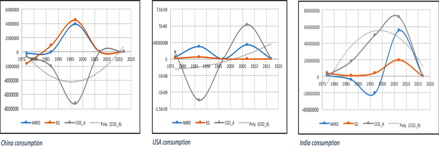
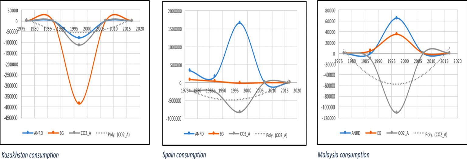
Fig. 6. High and low level of consumption. Note: high level consumption (China, USA and India) and low level (Kazakhstan, Spain and Malaysia)
5. Conclusions and policy implications
This research study assesses the relationship between the energy computation by Energy, Natural Gas, Nuclear Energy, Oil Gas and Coal, Renewable Energy and its effect on GDP in the period of 1968 and 2017 using a panel data set. The co-variance of GLM and stepwise regression were applied to investigate the relationship among an individual group of explanatory variables. After the Granger causality, variance analysis was used on the energy consumption and contribution of a relevant factor of production of electricity by the difference in sources and the intensity of CO2 emission in 24 (polluted) countries. It is significant that in each group there is a sign for a unidirectional relationship of the Granger causality in the energy consumption.
That Natural resources, use of energy, natural gas, electricity production by natural gas, coal rent, electricity production by coal rent, nuclear energy, production of electricity by nuclear energy, production of electricity by oil, gas and coal, electricity access, net saving and waste combustion, are not a Granger cause of energy; natural gas, carbon emission from solid fuel, green gas emission, intensity of CO2 and emission by manufacturing industries differed from earlier studies and specify that the level of growth of energy consumption precedes in polluted countries, which can be comprehended as a feature of economic growth. The negative results on economic sectors might be the cause of misused energy resources. The unidirectional causality runs from economic growth to energy consumption. The analysis estimation results show that the huge production of electricity from different sources that causes CO2 emissions and influences economic growth and validity has decreased after a continuous increase and steadying period. However, a positive unidirectional causality from 24 (polluted) countries’ energy consumption to economic development was detected, while a short-run bidirectional casualty exists among the above six groups of variables. These estimated results also showed some valuable strategy and implications as follows.
First, energy and natural gas intake policies should revised and changed in China, the USA, India, Russia, and Japan to reduce energy, natural gas and green gas consumption in the 6th (Next ten years) period and control the production of electricity by natural resources in group A, B, C, and D. However, the oil, gas and renewable energy consumption in Saudi Arabia, Iran, Korea, and China changed with new equips and policies to control the CO2 emissions and the production of electricity. Second, the Granger causality test results suggest a unidirectional causality from Energy, Natural Gas, Coal rent, Nuclear Energy Oil, Gas and Coal Renewable Energy consumption to economic growth. And the consequences of results impulse a response, the impact of 24 (polluted) countries energy consumption would at first increase then decrease, and the upcoming 6th and 7th periods would stabilize more with new changed strategies for control energy consumption. Third, a clean energy consumption role should endorsed in the above countries, so that energy environmental quality and affordability is enhanced and the ecosystem is secured in an upcoming period. Fourth, renewable energy by alternative means emits less carbon elements and controls the release of harmful gasses to the environment. Fifth, high-polluted countries should avoid high quantities of oil and gasses for development and introduce safe and controllable natural resources like solar and wind power. We find a unilateral causality in between energy consumption and economic growth. Therefore, the consumption of energy might be conductive of 24 (polluted) countries and better economic development, the consumption of energy face lifted and guaranteed, while we should limit the resources of countries. Thus, varying current consumption of the energy mix in above countries, and likewise promoting clean energy, is necessary for the coming generations.
Acknowledgement
This research is financed by the National Natural Science Foundation of China No: 71371087 of Jiangsu University. I appreciate my parent’s efforts and enthusiasm in my research, and I never ever neglect their consideration in my soul. Last I acknowledge my supporter and an admirer who offered me fortitude and leadership for justifying myself.
References
Acheampong, A. O. (2018). Economic growth, CO2 emissions and energy consumption: What causes what and where? Energy Economics, 74, 677-692. doi:https://doi.org/10.1016/j.eneco.2018.07.022
Alkhathlan, K., & Javid, M. (2015). Carbon emissions and oil consumption in Saudi Arabia. Renewable and Sustainable Energy Reviews, 48, 105-111. doi:https://doi.org/10.1016/j.rser.2015.03.072
Anandarajah, G., & Gambhir, A. (2014). India’s CO2 emission pathways to 2050: What role can renewables play? Applied Energy, 131, 79-86. doi:https://doi.org/10.1016/j.apenergy.2014.06.026
Aydin, M. (2019). The effect of biomass energy consumption on economic growth in BRICS countries: A country-specific panel data analysis. Renewable Energy, 138, 620-627. doi:https://doi.org/10.1016/j.renene.2019.02.001
Baek, J. C., Y.J. . (2017). Does Foreign Direct Investment Harm the Environment in Developing Countries? Dynamic Panel Analysis of Latin American Countries. Economies, 5(39). doi:https://doi.org/10.3390/economies5040039
Boden, T. A., G.Marland, & R.J.Andres. (2011). Global, Regional, and National Foossil-Fuel CO2 Emission. Retrieved from USA:
Cai, Y., Sam, C. Y., & Chang, T. (2018). Nexus between clean energy consumption, economic growth and CO2 emissions. Journal of Cleaner Production, 182, 1001-1011. doi:https://doi.org/10.1016/j.jclepro.2018.02.035
Chen, J., Shi, Q., Shen, L., Huang, Y., & Wu, Y. (2019). What makes the difference in construction carbon emissions between China and USA? Sustainable Cities and Society, 44, 604-613. doi:https://doi.org/10.1016/j.scs.2018.10.017
Cheng, C., Ren, X., Wang, Z., & Yan, C. (2019). Heterogeneous impacts of renewable energy and environmental patents on CO2 emission - Evidence from the BRIICS. Science of The Total Environment, 668, 1328-1338. doi:https://doi.org/10.1016/j.scitotenv.2019.02.063
Cheng, Z., Wang, J., Wei, S., Guo, Z., Yang, J., & Wang, Q. (2017). Optimization of gaseous fuel injection for saving energy consumption and improving imbalance of heat distribution in iron ore sintering. Applied Energy, 207, 230-242. doi:https://doi.org/10.1016/j.apenergy.2017.06.024
Chong, C. H., Tan, W. X., Ting, Z. J., Liu, P., Ma, L., Li, Z., & Ni, W. (2019). The driving factors of energy-related CO2 emission growth in Malaysia: The LMDI decomposition method based on energy allocation analysis. Renewable and Sustainable Energy Reviews, 115, 109356. doi:https://doi.org/10.1016/j.rser.2019.109356
Dong, F., Wang, Y., Su, B., Hua, Y., & Zhang, Y. (2019). The process of peak CO2 emissions in developed economies: A perspective of industrialization and urbanization. Resources, Conservation and Recycling, 141, 61-75. doi:https://doi.org/10.1016/j.resconrec.2018.10.010
Dong, K., Sun, R., & Dong, X. (2018). CO2 emissions, natural gas and renewables, economic growth: Assessing the evidence from China. Science of The Total Environment, 640-641, 293-302. doi:https://doi.org/10.1016/j.scitotenv.2018.05.322
Emirmahmutoglu, F., & Kose, N. (2011). Testing for Granger causality in heterogeneous mixed panels. Economic Modelling, 28(3), 870-876. doi:https://doi.org/10.1016/j.econmod.2010.10.018
Etemad, B., J.Luciani, P.Bairoch, & J.C.Toutian. (1991). World Energy Production 1800-1985. Retrieved from Librarie DROZ, Switzerland.:
Fadiran, G., Adebusuyi, A. T., & Fadiran, D. (2019). Natural gas consumption and economic growth: Evidence from selected natural gas vehicle markets in Europe. Energy, 169, 467-477. doi:https://doi.org/10.1016/j.energy.2018.12.040
González, R. M., Marrero, G. A., Rodríguez-López, J., & Marrero, Á. S. (2019). Analyzing CO2 emissions from passenger cars in Europe: A dynamic panel data approach. Energy Policy, 129, 1271-1281. doi:https://doi.org/10.1016/j.enpol.2019.03.031
Gupta, N. C., Jain, V. K., & Bansal, N. K. (1995). CO2 reduction potential through non-conventional energy sources in India. Energy, 20(6), 549-553. doi:https://doi.org/10.1016/0360-5442(94)00093-I
Hao, Y., Wang, L. o., Zhu, L., & Ye, M. (2018). The dynamic relationship between energy consumption, investment and economic growth in China’s rural area: New evidence based on provincial panel data. Energy, 154, 374-382. doi:https://doi.org/10.1016/j.energy.2018.04.142
Hardin, J. W. a. J. M. H. (2007 ). Generalized Linear Models and Extensions (Second ed.).
Herrerias, M. J., Joyeux, R., & Girardin, E. (2013). Short- and long-run causality between energy consumption and economic growth: Evidence across regions in China. Applied Energy, 112, 1483-1492. doi:https://doi.org/10.1016/j.apenergy.2013.04.054
Hosseini, S. M., Saifoddin, A., Shirmohammadi, R., & Aslani, A. (2019). Forecasting of CO2 emissions in Iran based on time series and regression analysis. Energy Reports, 5, 619-631. doi:https://doi.org/10.1016/j.egyr.2019.05.004
Jeong, K., Hong, T., & Kim, J. (2018). Development of a CO2 emission benchmark for achieving the national CO2 emission reduction target by 2030. Energy and Buildings, 158, 86-94. doi:https://doi.org/10.1016/j.enbuild.2017.10.015
Jiang, X.-t., Wang, Q., & Li, R. (2018). Investigating factors affecting carbon emission in China and the USA: A perspective of stratified heterogeneity. Journal of Cleaner Production, 199, 85-92. doi:https://doi.org/10.1016/j.jclepro.2018.07.160
Jin, T., & Kim, J. (2018). What is better for mitigating carbon emissions – Renewable energy or nuclear energy? A panel data analysis. Renewable and Sustainable Energy Reviews, 91, 464-471. doi:https://doi.org/10.1016/j.rser.2018.04.022
Kang, S. H., Islam, F., & Kumar Tiwari, A. (2019). The dynamic relationships among CO2 emissions, renewable and non-renewable energy sources, and economic growth in India: Evidence from time-varying Bayesian VAR model. Structural Change and Economic Dynamics, 50, 90-101. doi:https://doi.org/10.1016/j.strueco.2019.05.006
Kao C, C. B. (1995). On the estimation and inference of a cointegrated regression in
panel data when the cross-section and time-series dimensions are compa-rable. . Syracuse University: Department of Economics, .
Karney, D. H. (2019). Electricity market deregulation and environmental regulation: Evidence from U.S. nuclear power. Energy Economics, 104500. doi:https://doi.org/10.1016/j.eneco.2019.104500
Ketenci, N. (2018). The environmental Kuznets curve in the case of Russia. Russian Journal of Economic, 4(3), 249-265.
Kharbach, M., & Chfadi, T. (2018). Oil prices and electricity production in Morocco. Energy Strategy Reviews, 22, 320-324. doi:https://doi.org/10.1016/j.esr.2018.10.006
Kong, Y., & Khan, R. (2019). To examine environmental pollution by economic growth and their impact in an environmental Kuznets curve (EKC) among developed and developing countries. PloS one, 14(3). doi:https://doi.org/10.1371/journal.pone.0209532
Kumar, S., & Sinha, S. (1995). Non-CO2-emitting renewable energy sources in India: Paths, realisable potential and requirement of industry related forestry pattern. Energy Conversion and Management, 36(6), 885-888. doi:https://doi.org/10.1016/0196-8904(95)00145-4
Li, Z.-G., Cheng, H., & Gu, T.-Y. (2019). Research on dynamic relationship between natural gas consumption and economic growth in China. Structural Change and Economic Dynamics, 49, 334-339. doi:https://doi.org/10.1016/j.strueco.2018.11.006
Liang, T., Chai, J., Zhang, Y.-J., & Zhang, Z. G. (2019). Refined analysis and prediction of natural gas consumption in China. Journal of Management Science and Engineering. doi:https://doi.org/10.1016/j.jmse.2019.07.001
Lin, J., Fridley, D., Lu, H., Price, L., & Zhou, N. (2018). Has coal use peaked in China: Near-term trends in China’s coal consumption. Energy Policy, 123, 208-214. doi:https://doi.org/10.1016/j.enpol.2018.08.058
McCullagh, P., and J. A. Nelder. (1989). Generalized Linear Models (Second ed.). London: Chapman & Hall.
McGee, J. A., & Greiner, P. T. (2019). Renewable energy injustice: The socio-environmental implications of renewable energy consumption. Energy Research & Social Science, 56, 101214. doi:https://doi.org/10.1016/j.erss.2019.05.024
Mezghani, I., & Ben Haddad, H. (2017). Energy consumption and economic growth: An empirical study of the electricity consumption in Saudi Arabia. Renewable and Sustainable Energy Reviews, 75, 145-156. doi:https://doi.org/10.1016/j.rser.2016.10.058
Morales Pedraza, J. (2019). Chapter 4 - Current Status and Perspective in the Use of Coal for Electricity Generation in the North America Region. In J. Morales Pedraza (Ed.), Conventional Energy in North America (pp. 211-257): Elsevier.
Ohashi, M., Maekawa, Y., Hashimoto, Y., Takematsu, Y., Hasin, S., & Yamane, S. (2017). CO2 emission from subterranean nests of ants and termites in a tropical rain forest in Sarawak, Malaysia. Applied Soil Ecology, 117-118, 147-155. doi:https://doi.org/10.1016/j.apsoil.2017.04.016
P., P. (2004). Panel cointegration: Asymptotic and Finite Sample Properties of Pooled Time Series Tests with an Application to the PPP Hypothesis. Econometric theory, 3, 579-625.
Pao, H.-T., & Tsai, C.-M. (2011). Multivariate Granger causality between CO2 emissions, energy consumption, FDI (foreign direct investment) and GDP (gross domestic product): Evidence from a panel of BRIC (Brazil, Russian Federation, India, and China) countries. Energy, 36(1), 685-693. doi:https://doi.org/10.1016/j.energy.2010.09.041
Shan, Y., Guan, D., Meng, J., Liu, Z., Schroeder, H., Liu, J., & Mi, Z. (2018). Rapid growth of petroleum coke consumption and its related emissions in China. Applied Energy, 226, 494-502. doi:https://doi.org/10.1016/j.apenergy.2018.06.019
Solaymani, S. (2019). CO2 emissions patterns in 7 top carbon emitter economies: The case of transport sector. Energy, 168, 989-1001. doi:https://doi.org/10.1016/j.energy.2018.11.145
Uribe, J. M., Guillen, M., & Mosquera-López, S. (2018). Uncovering the nonlinear predictive causality between natural gas and electricity prices. Energy Economics, 74, 904-916. doi:https://doi.org/10.1016/j.eneco.2018.07.025
Valadkhani, A., Nguyen, J., & Bowden, M. (2019). Pathways to reduce CO2 emissions as countries proceed through stages of economic development. Energy Policy, 129, 268-278. doi:https://doi.org/10.1016/j.enpol.2019.02.024
Wang, C., Zhang, L., Zhou, P., Chang, Y., Zhou, D., Pang, M., & Yin, H. (2019). Assessing the environmental externalities for biomass- and coal-fired electricity generation in China: A supply chain perspective. Journal of Environmental Management, 246, 758-767. doi:https://doi.org/10.1016/j.jenvman.2019.06.047
Wolde-Rufael, Y., & Menyah, K. (2010). Nuclear energy consumption and economic growth in nine developed countries. Energy Economics, 32(3), 550-556. doi:https://doi.org/10.1016/j.eneco.2010.01.004
Xu, B., & Lin, B. (2019). Can expanding natural gas consumption reduce China’s CO2 emissions? Energy Economics, 81, 393-407. doi:https://doi.org/10.1016/j.eneco.2019.04.012
Xu, G., Schwarz, P., & Yang, H. (2019). Determining China’s CO2 emissions peak with a dynamic nonlinear artificial neural network approach and scenario analysis. Energy Policy, 128, 752-762. doi:https://doi.org/10.1016/j.enpol.2019.01.058
Xu, X., Huo, H., Liu, J., Shan, Y., Li, Y., Zheng, H., . . . Ouyang, Z. (2018). Patterns of CO2 emissions in 18 central Chinese cities from 2000 to 2014. Journal of Cleaner Production, 172, 529-540. doi:https://doi.org/10.1016/j.jclepro.2017.10.136