Ekonomika ISSN 1392-1258 eISSN 2424-6166

2020, vol. 99(1), pp. 6–25 DOI: https://doi.org/10.15388/Ekon.2020.1.1

The Relationships between Economic growth, Energy Efficiency and CO2 Emissions: Results for the Euro Area¹

Dr. Angelė Kėdaitienė
Lulea Technical University,
Sweden and Vesalius College, Belgium
Email: angele.kedaitiene@outlook.com

Dr. Violeta Klyvienė
European Parliament, Belgium
Email: violeta.klyviene@europarl.europa.eu

Abstract. The article aims at ascertaining the relationship between indicators affecting the green economic growth of the Eurozone countries. Despite extensive research, scientists have not yet found a clear answer as to whether economic growth and climate change mitigation can be aligned. Another important aspect of the study was to investigate the possible effect of environmental policies on macroeconomic variables such as GDP, investment, employment, and trade. The authors of the article applied the PVAR econometric model to measure the impact of energy consumption, CO2 emissions, and some of the macroeconomic indicators on GDP growth in 19 countries of the Eurozone for years 2000–2016.
Based on the results, we cannot yet state explicitly that economic growth in the Eurozone countries has been decoupled from climate change mitigation; however, green transition is on the right track.
JEL Codes: O44 (Environment and growth), Q5 (Environmental economics), E6 (Macroeconomic policy).
Keywords: Green economic growth, GDP growth, CO2 emissions, energy efficiency, macroeconomic indicates.

Received: 05/04/2020. Revised: 22/04/2020. Accepted: 23/04/2020
Copyright © 2020 Angele Kedaitiene, Violeta Klyviene. Published by Vilnius University Press
This is an Open Access article distributed under the terms of the Creative Commons Attribution Licence, which permits unrestricted use, distribution, and reproduction in any medium, provided the original author and source are credited.

Note: Views of the authors presented in the article represent personal opinion only, not that of the European Parliament as the institution.

Introduction

Climate change policies, movements, and research are rapidly gaining momentum around the globe. The European Union aims at becoming a CO2 emissions-free zone by 2050. Chinese National People’s Congress, which took place in March 2019, labelled mitigation of the climate change as a major policy priority in the coming years. School and youth climate strikes, led by the Swedish activist Greta Thunberg, have taken place around the globe.

At the same time, economies around the world strive for economic growth, employment, and improved living standards. Countries are still feeling the consequences of the last economic crisis, while the new recession due to COVID-19 is already on the horizon. Economic growth is an important issue here, also taking into account that climate change mitigation needs budgetary resources. In this respect, aligning economic growth with climate change mitigation polices is a priority in countries striving for answers.

The article aims at ascertaining the relationship between indicators affecting the green economic growth of the Eurozone countries. The discussion around climate change mitigation and the countries’ economic growth, as well as the possible decoupling of these processes, has been on the research and policy agenda of the interested parties for a number of years, if not decades.

Despite extensive research, scientists have not yet found a clear answer as to whether economic growth and climate change mitigation can be aligned. The results depend on data samples, countries covered, and methods applied; they also depend on national governmental policies.

The article’s main hypothesis relates to the assumptions that:

• despite deploying climate change mitigation polices, the Eurozone economies have not yet succeeded in fully decoupling climate change mitigation from economic growth;
• while deploying climate change mitigation polices, the Eurozone economies did already succeed in decoupling climate change mitigation from the economic growth.

The hypothesis has been tested by an empirical analysis using two data sets with different variables. The first assumption has been confirmed – that despite deploying climate change mitigation polices, the Eurozone economies have not yet succeeded in fully decoupling climate change mitigation from economic growth.

The article is based primarily on the attempt to ascertain results while using only three basic variables: GDP growth, energy efficiency, and CO2 emissions. The results of the second attempt using six variables have been used for the robustness checks, although they also reflect on the macroeconomic channels to be used for the transmission of the climate change mitigation polices to the economy at large.

Chapter 1 of the article provides a brief literature review of the relationship between economic growth and climate change mitigation, and between energy consumption and CO2 emissions.

Chapter 2 describes European Union’s recent initiatives in relation to climate change mitigation, particularly those related to the President of the European Commission Ursula von der Leyen’s Green Deal initiative.

Chapter 3 analyzes the relationship between energy efficiency and economic growth.

Chapter 4 describes the data sets and econometric methods used (PVAR model). In the research, we used data for 19 Eurozone countries for years 2000–2016. The PVAR model was chosen because of its proven ability to measure ambiguity relationships, especially when the time frames are relatively short.

Chapter 5 analyzes the research results implying that we cannot yet state explicitly that economic growth in the Eurozone countries has been decoupled from the climate change mitigation; however, green transition is on the right track.

1. Climate change mitigation and economic growth

2018 Nobel Prize in economics (given to Nordhaus and Romer), granted for pioneering research on climate change and economic growth, underlines the importance of further research—taking into account the IPCC report on 1.5°C (M. Allen, Chen, Jacob, 2018)—urging countries to take immediate action in the area of climate change mitigation. COP24 in Katowice agreed on the rule book to implement the Paris climate change agreement, although climate experts agree that the ambition is far from sufficient to prevent global warming below 2°C.

For a long time, Nordhaus has emphasized economic growth over climate change mitigation. In the 1990s, Nordhaus invented the first models explaining the relationship between economic growth and CO2 emissions, which the IPCC have used for econometric simulations up to now. These models showed that a rapid reduction of CO2 emissions to avoid climate catastrophe, by applying relevant polices such as a high tax on carbon, would significantly slow down the rate of economic growth. In his famous article “To slow or not to slow” (1991), Nordhaus argued for economic growth—to focus on GDP growth even if it means a future climate catastrophe. In his view, future generations will then be much richer than we are now and therefore better able to manage the problem even if the temperature rises by 3.5°C above the pre-industrial levels. These arguments resulted in economists and policymakers sticking to the status quo and delaying key decisions. This largely explains why, nearly 30 years after the first IPCC report was published, global emissions are still going up and why even with the Paris climate agreement in place, the world is still heading for a temperature above 3°C.

However, Nordhaus was not the only one to influence the public debate on the issue. For example, the relationship between economic growth and environmental indicators was the major topic of The Limits to Growth (Meadows, Randers, Behrens, 1972), a debate report by the Club of Rome. According to the report, and contrary to Nordhaus, economic growth meant greater negative environmental impacts, which could be reduced by a slowdown in population and consumption growth, i.e., by de-growth. The mainstream view was that the environment and economy were two conflicting goals.

By the late 1980s, with the emergence of the sustainable development concept, the invention of empirical models (so-called environmental Kuznets curves or EKCs) shifted the relationship between the environment and economics while stating that they show an inverted U-shape relation, with pollution or other forms of degradation rising in the early stages of economic development and falling in the latter.

A well-known professor of competitiveness and strategy, Michael Porter, stated already in 1991 that economic growth could get hand in hand with environmental protection. Per him, and his later co-author van der Linde, the pollution is the waste of resources and a reduction of pollution may lead to an improvement in the productivity. More stringent but properly designed environmental regulations can “trigger innovation [broadly defined] that may partially or more than fully offset the costs of complying with them” (Porter and van der Linde, 1995). This became known as the Porters Hypothesis, which has raised some debate among scholars of economy.

Can we still have economic growth and stay under 1.5 C degrees? The IPCC states clearly that we need to completely decarbonize the global economy by the middle of the century. However, the global economy will nearly triple in size during that same period, and it will be difficult enough to decarbonize the existing global economy so quickly.

Jeffrey Sachs (2019), a famous US climate change economist, has recently been rather positive about the green transition, stating that “the solution to human-induced climate change is finally in clear view. Thanks to rapid advances in zero-carbon energy technologies, and in sustainable food systems, the world can realistically end greenhouse-gas emissions by mid-century at little or no incremental cost, and with decisive benefits for safety and health.” According to Sachs, the main obstacle are the politicians continuously favoring the fossil-fuel industry due to a lack of knowledge or lobbying.

The COVID-19 pandemic of 2020 could strengthen attention given to climate change mitigation. Governments may increase their role, and public policies may prioritize public interest. It could lead to increased international cooperation, including the area of climate change mitigation.

2. Climate change as a European Union policy

The European Union is climate-ambitious—it aims at leading the world in climate change mitigation.

In November 2018, the European Commission set an agenda for the European Union to become carbon neutral by 2050. The recent European Commission, operational as of 1 December 2019, has proceeded with this ambitious goal while putting forward the Green Deal for Europe (2019) and the European Climate Law, both providing the polices and legal framework to reach the zero carbon emissions goal. According to the President of the European Commission, Ursula von der Leyen,2 “the European Green Deal is our new growth strategy – for a growth that gives back more than it takes away. It shows how to transform our way of living and working, of producing and consuming so that we live healthier and make our businesses innovative. We can all be involved in the transition and we can all benefit from the opportunities. We will help our economy to be a global leader by moving first and moving fast. We are determined to succeed for the sake of this planet and life on it – for Europe’s natural heritage, for biodiversity, for our forests and our seas. By showing the rest of the world how to be sustainable and competitive, we can convince other countries to move with us.”

Furthermore, according to Jeffrey Sachs (2019), “the European Green Deal announced by the European Commission is the first comprehensive plan to achieve sustainable development in any major world region. As such, it becomes a global benchmark – a ‘how-to’ guide for planning the transformation to a prosperous, socially inclusive, and environmentally sustainable economy.”

However, this will require efforts, first of all agreements with the national governments, with the societies, and with the private sectors. It will also require massive investments, done through the Sustainable Europe Investment Plan and by transforming some departments of the European Investment Bank into a Climate Bank. This will facilitate a €1 trillion of investment during the next 10 years.

Finally, emissions must have a price that changes our behavior. To complement this work and to ensure that EU companies can compete on an equal conditions-based playing field, the European Commission would consider introducing a relevant carbon border adjustment mechanism to avoid carbon leakage. However, discussions leading to a concrete proposal might take years. Not all scientists and policymakers agree on the relevance of such mechanism.

The Director General of DG CLIMA of the European Commission, Mr. Mauro Petriccione, also agreed that the next 10 years (two terms of the European Commission) would be decisive for the green transformation to be placed at the heart of EU polices. In this sense, economic stability is of the utmost importance, along with the transformation of the existing economic model and technological transformation. Boosting the research expenditure is needed right now.

These are some ideas to be put into practice at the European Union level although the major work in reducing CO2 emissions is to be done by member states. The European Union does not have a common climate policy yet. Member states vary in their climate approaches. Some are strongly ahead: Germany, France, the Scandinavian countries, Spain, Portugal, Lithuania, Latvia, Bulgaria, and Romania; others (Visegrad 4, especially Poland) prefer cautious polices on climate mitigation while voting against the EU climate ambition of the carbon neutral EU-2050 at the EU Councils.

The recent COVID-19 pandemic could alter the EU’s plans in two ways. First of all, many countries—including China—have recorded lower emission levels due to decreased economic activity; data demonstrating this decoupling is not clear yet. Second, in order to overcome the economic recession, both the European Commission and the member states will be directing significant financial resources to stimulate the economies. This means that less will be left to combat climate change. On the other hand, since the economy stimulus packages would be conditioned toward the green transition related expenditures, this would make the case of fostering the green transition in EU.

3. Energy efficiency and economic growth

A big part of the debate focuses around the impact of energy use, or more specifically energy efficiency measures, on the EU countries’ economic growth. Assuming that higher efficiency leads to higher growth, it would mean that the decoupling of economic growth from climate change mitigation is under way.

Academic literature informs the debate on energy use as input of production, including that it is virtually impossible to reduce energy use to the extent of decoupling climate change from economic growth. Theoretically, the main problem is the mainstream neoclassical economic growth theory by the Nobel prizewinning economist Robert Solow, which does not take into account the role of resources in the economy (Solow, 1956).

According to the neoclassical growth theory, the only driver of continuing economic growth is technological progress. As the level of technological knowledge rises, the functional relationship between productive input and output changes.

The limitations of this consideration have been the subject of academic dispute, based on the so-called biophysical theory of the role of energy (Stern, Cleveland, 2004). Two laws could be applied here. According to the first law of thermodynamics, in order to obtain material output, greater or equal quantities of materials must enter the production process as the input. According to the second law of thermodynamics, there must be a minimum quantity of energy, which is required for transformation of the materials. In this respect, there should be limits to the substitution of other materials for energy.

Back in year 1974, in a paper published in a special issue of the Review of Economic Studies, Solow has demonstrated how sustainability could be achieved with finite and non-renewable natural resources. Although during the same year, in a special issue of the same journal, Solow’s fellow colleagues, Dasgupta and Heal, showed that with any constant discount rate, the so-called optimal growth path also leads to the eventual depletion of the natural resource and collapse of the economy. These findings, as well as some other similar developments, have led to the conclusion that substitution and technical change can facilitate the decoupling of the economic growth from the use of resources and from the environmental conditions, which could be replaced either by the abundant substitutes, or by some equivalent forms of capital, such as machines and factories, or by people. In this way, neoclassical economists typically assume that sustainability is technically feasible unless proven otherwise. Then, the focus is on institutional arrangements, which might lead to sustainability.

According to Stern and Cleveland (2004) and from the neoclassical perspective, in order to explain the factors behind weaker or stronger linkage between energy use and economic activity, a general production function can be represented as follows:

(Q1….Qm) = f (A , X1…Xn, E1….Ep) (1)

where Q represents the outputs (goods and services), X – the inputs (capital, labour, etc.), E – the energy inputs (coal, oil, etc.), and A is the indicator of the state of technology, according to the denomination of the total factor productivity. The functional relationship between energy and the output could be altered by availability of the substitution between energy and other inputs, by the fact and speed of the technological change, by changes in the components of the energy input, and by changes in the components of output.

There is a large number of differing empirical studies that investigate the causal links between energy consumption and economic growth, first done by Kraft and Kraft (1978). Some of the studies focus on the total energy consumption and on particular groups of countries (South Asia, OECD, G20, North America, etc.). Others analyze the energy usage by energy source, such as electricity, coal, nuclear, and renewable resources (Chiou-Wei et al., 2008; Akinlo, 2009; Apergis and Payne, 2009b; Ghosh, 2009; Eggoh et al., 2011; Chu and Chang, 2012; Dagher and Yacoubian, 2012; Abbas and Choudhury, 2013; Bozoklu and Yilanci, 2013; Dergiades et al., 2013; Yıldırım et al., 2014). There are studies that assess the impact of the development level and income in the energy-growth nexus (Chontanawat et al., 2008; Huang et al., 2008; Joyeux and Ripple, 2011) reporting different results among developed and developing countries and proving the effects of the environmental Kuznetz curve. A paper by Grossman and Krueger (1991) paved the way for the empirical testing of the environmental Kuznetz curve and allowed numerous studies to explore linear and non-linear relationships between economic activity and emissions. Dinda (2004), Stern (2004), Kijima et al. (2010), Furuoka (2015), and Al-Mulali et al. (2015) provide an exhaustive list of studies in their literature reference lists. Findings are inconclusive and country- or region-specific. Finally, there are studies that use a unified framework to identify the links between energy consumption, emissions, and economic growth (Soytas et al., 2007; Ang, 2008; Apergis and Payne, 2009a; Soytas and Sari, 2009; Zhang and Cheng, 2009; Halicioglu, 2009). This link is extremely important for the policy decision-makers. However, even in this more holistic approach, results often remain contradictory.

The majority of these studies provide evidence based on total energy consumption and focus on small groups of countries (ASEAN, BRICS, etc.). Furthermore, these studies focus mainly on the nexus of economic activity, energy consumption, and environmental waste in developing economies (where economic growth has caused environmental concerns) and stress the necessity of identifying efficient ways for energy consumption and growth (Zhang, 2003; Wang et al., 2015; Wang and Feng, 2015a; Zhang and Wang, 2014).

The main conclusion of these studies is that the results are rather mixed. Potential explanations for the conflicting results could be, among others, the different time periods and country-sample data, different econometric approaches, and/or the omitted variables bias. In addition, the majority of these studies are based on a static, not dynamic, analysis of aggregated (total) data of energy consumption, and/or they focus on a small group of countries.

Chapter 4. Data and methods

4.1. Statistical data

To test the hypothesis of the research, we have used the Eurostat data for the years 2000–2016 for the following indicators:

• GDP per capita in PPP (GDP)
• Final energy consumption, tones of oil equivalent per capita (EC)
• CO2 emissions, in tonnes per capita (CO2)
• Employment as share of persons between the age of 20 to 64 years (LF)
• Exports and Imports as share of GDP (EXP)
• Investments as share of GDP (INV)

The indicators represent the effects of various climate change mitigation polices on the economic growth of the countries. The investigations are based on data from 19 Eurozone countries.

4.2. PVAR model

We have chosen the PVAR (panel vector auto regression) model as the method to prove the relationships. This is one of the most commonly applied analysis methods used to explore the relationship between energy consumption indicators and economic growth.

There are several advantages of using a PVAR methodology.

First, PVARs are extremely useful when there is little or ambiguous theoretical information regarding the relationships among the variables. The literature review did confirm that various studies have found varying and sometimes even conflicting results.

Second, and more importantly, PVARs are explicitly designed to address the endogeneity problem, which is one of the most serious challenges of the empirical research on energy consumption and economic growth. PVARs help minimize the endogeneity problem by treating variables as potentially endogenous.

Third, impulse response functions based on PVARs can account for any delayed effects on the variables under consideration and thus determine whether the effects between energy consumption, economic growth, and CO2 emissions are short-term, long-term, or both. We have analyzed the panel impulse response function to examine both the short-term and the long-term interdependencies in the energy-growth-emissions nexus.

Fourth, a PVAR analysis allows us to capture country-fixed effects that may affect energy consumption and growth as well as global time effects that affect all countries in the same period.

Finally, PVARs can be effectively employed with relative short-time series due to the efficiency gained from the cross-sectional dimension.

Following the recent empirical literature (Sumskis and Giedraitis, 2015; Antonakakis et al., 2017; Caruso et al., 2020) that we have used for the panel VAR, which was originally developed by Holtz-Eakin et al. (1988), we propose the following:

X_s =Γ(L) X_i,t + d_i + ε_i,t (2)

Where i = 1, 19 cross-section data series; X_i,t is a 1x3 vector of three key endogenous variables: a) GDP per capita, b) energy consumption, c) CO2 emission, expressed as first difference of the natural logarithms; Γ(L) is the lag operator; d_i denotes the fixed effect; and ε_i,t denotes the vector of residuals. We estimated the coefficients by using GMM routine (Holtz-Eakin et al., 1988; Love and Zicchino, 2006; Antonakakis et al., 2017).

The first step of the PVAR model specification is testing for data stationarity. The authors have selected 4 different augmented tests: 1) Levin, Lin, and Chu (LLC), 2) Im, Pesaran and Shin (IPS), 3) Dickey-Fuller (ADF), 4) Phillips-Perron (PP). All the tests analyze 2 different processes in observed data series: random walk and random walk with intercept and trend. It is evident that all of the variables are stationary in the first differences while the level results indicate the presence of a unit root (see Annex, Table 1). In the second step, the lag length selections were made according to selection criteria tests for lags based on LR (sequential modified Likelihood Ratio test statistic); AIC (Akaike information criterion), SC (Schwarz information criterion); HQ (Hannan-Quinn information criterion). We have also selected 2-lags specification in order not to over-parameterize the model (see Annex, Table 2 and 3).

4.3. Granger causality tests

In order to analyze if there are any causality relations in the PVAR model between energy consumption, CO2 emissions, and macroeconomic variables such as investments, employment, external trade, and deflator, we have performed Granger causality Wald tests.

The null hypothesis of a Granger causality test is formulated when the explanatory variable does not provide for Granger causality on the dependent variable. Table 1 depicts the null hypotheses and implied restrictions that were set for Granger causality tests to evaluate the test results. All tested variables are in the stationary form as described previously. Results show that there is Granger causality between energy consumption as independent variable to GDP and to CO2 as the dependent variables at 5% significance level. Those results are in line with most of the economic literature.

Table 1. Granger causality Wald test results

Variables	∆ln GDP	∆ ln EC	∆ ln CO2
∆ln GDP	-	7.4	9.7
∆ln EC	18.5*	-	19.2*
∆ln CO2	10.5	7.4	-

Note:* represents at least 5% significance levels, column variables are dependent variables; (∆ln) denotes first difference of the natural logarithms
Source: Authors’ Calculations

Causality tests, by their nature, cannot describe whether relations between variables are positive or negative, how much time it takes for the effects to be initiated, and how long such effects could last.

Thus, the final step of the PVAR model analysis is to calculate the impulse-response functions and variance decompositions in order to demonstrate and graphically reproduce the significance and magnitude of relationships between the variables. The analysis of impulse-response functions is presented in the analysis chapter.

Chapter 5. Data analysis

5.1. Secondary data analysis

We will briefly analyze the main developments related to energy efficiency and CO2 emissions.

The debates concerning the energy efficiency trends in the developed economies are without end. According to Eurostat, primary energy consumption in 2005–2016 decreased just by 10% on average. However, the change was rather uneven. In some EU member states, such as Estonia and Poland, this consumption even increased. The most savings were observed in Lithuania and Greece.

As regards other European countries, energy consumption increased even in traditionally green Nordic countries such as Norway and Iceland; in Iceland, it almost doubled. The uneven path empirically suggests that energy consumption depends on a number of factors—not just on energy efficiency and economic growth but also structural changes as well as institutional and governmental policies. Also, the Nordic countries have to spend a lot of energy on the colder winters. However, most of this period was affected by the financial and economic crisis, with austerity policies in place that could lead to energy savings and provide for policy-based turbulences. Despite that, GDP grew during the period of 2005–2016. Since the energy consumption decreased on average, it can be concluded that there might have been some decoupling of economic output and resources, which could also mean the less restrictive economic growth.

The brief secondary data analysis of the gross energy consumption per capita for Eurozone countries, performed using the different data set, also showed that consumption went down during the decade. At the same time, even similar economic-zone countries demonstrated a huge variety of data: Malta was the biggest consumer of energy, along with Germany, Ireland, Austria, and the Netherlands, while Lithuania and Spain consumed less. Germany, Ireland, and Austria have large industries; Malta’s consumption could be driven by people having to use private cars to commute as there is very little public transport. In recent years, the Lithuanian government has paid sufficient attention toward increasing energy efficiency while changing technologies, developing a less energy-intensive service industry, encouraging the renovation of houses, and driving public transport and bike use.³

CO2 emissions per capita also vary across the Eurozone countries—Luxembourg, Estonia, Netherlands, and Germany emit the most, while Lithuania, Latvia, and Malta emit the least. The difference between the highest and lowest emitters is around 4–5 times, which is enormous. The fact that, during the decade, CO2 emissions decreased just a little, and that energy consumption per capita and CO2 emissions per capita correlate just for some countries, has driven us to the conclusion that reducing CO2 emissions depends on a particular national policy mix. The fact of Luxembourg being the highest emitter and energy consumer per capita can be explained by the presence of ironworking industry in the country, which has not yet technologically transformed to the extent of being green.

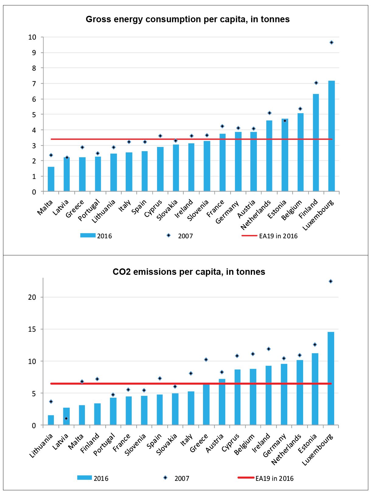
Figure 1. Energy consumption and CO2 emissions per capita in Eurozone countries

Source: Eurostat, author’s calculations

5.2. PVAR results analysis

In order to examine how a shock of one variable affects another variable and how long the effect lasts, we have utilized a generalized impulse response function analysis (Koop et al., 1996).

Both energy consumption and CO2 emissions demonstrate the significant impacts upon GDP per capita. Results of shocks presented in Figure 3 demonstrate that both energy consumption per capita and CO2 emissions per capita have short-term positive impact on GDP per capita, although this trend quickly becomes negative with the effects of around 3 years after the shock. The output gap driven by higher energy consumption and higher CO2 emissions might be linked to a number of factors, such as productivity decline, less efficiency, higher taxes, higher energy and production costs in general, social welfare losses, etc. CO2 emissions react slightly positively over the entire period to both the increase in energy consumption and to GDP growth, a logical reaction showing the decoupling yet to come. Energy consumption reacts slightly positively to the increase in CO2 emissions.

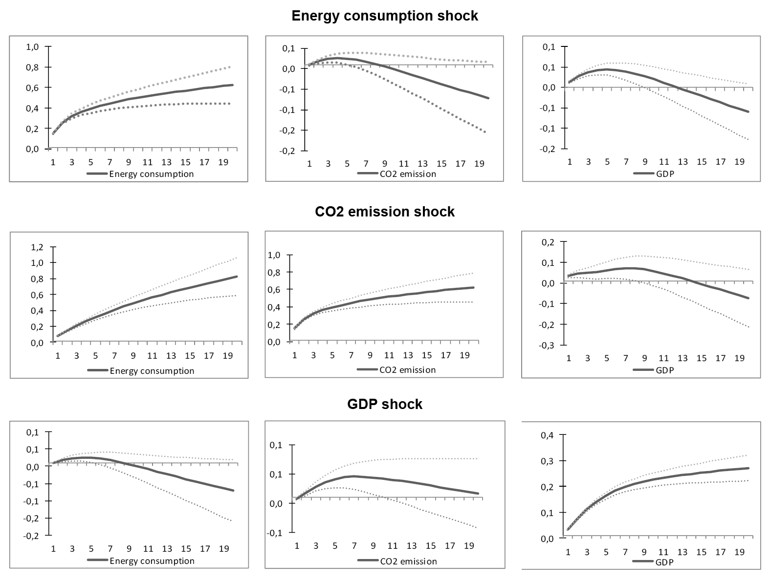
Figure 2. Accumulated generalized impulse response functions for PVAR

Source: Authors’ calculations.

What does it mean for policymakers? In principle, it means that the Eurozone is on the right track for the green transition. A climate policy that seeks to reduce energy consumption and CO2 emissions results in output loss that is temporary and marginal. This output gap is brief and lasts for about 3 years, so climate change mitigation is not going to affect GDP negatively over the longer period of time. Furthermore, the temporary output gap is very small, although it could be larger if other shocks (e.g., shock on labour, foreign trade, or investments) are included in the analysis.

5.3. Robustness checks

We have performed a variety of robustness checks for our baseline 3 variable-based PVAR model, as envisaged by the theory. Furthermore, we have performed PVAR estimates by including additional variables for 2000–2016, which aims to check the validity of the earlier results. The additional variables for the Eurozone include the following:

• GDP per capita in PPP (GDP)
• Final energy consumption, tonnes of oil equivalent per capita (EC)
• CO2 emissions, in tonnes per capita (CO2)
• Employment as share of persons aged 20 to 64 (LF)
• Exports and Imports as share of GDP (EXP)
• Investments as share of GDP (INV)

The results in Table 2 below show that there is a bi-directional Granger causality between GDP per capita and energy consumption at the 5% significance level in the Eurozone countries. The rest of the statistically significant bi-directional connections run from the energy consumption to foreign trade, employment, and investments indicators. The CO2-dependent variable significantly affects just the energy consumption.

Table 2. Results of the Granger causality Wald test

Variables	∆ln GDP	∆ln EC	∆ln CO2	∆ln EXP	∆ln LF	∆ln INV
∆ln GDP	-	25.5*	9,3	29.6*	31.2*	39.7*
∆ln EC	20.9*	-	10.8*	12.1*	18.9*	5.6
∆ln CO2	7.9	9.7	-	5.7	18.1*	2.6
∆ln EXP	34.1*	12.2*	8.2	-	17.0*	19.0*
∆ln LF	13.4*	18.7*	8.2	5.7	-	6.2
∆ln INV	7.3	17.2*	2.6	3.9	13.6*	-

Note:* represents at least 5% significance levels, column variables define row variables; (∆ln) denotes first difference of the natural logarithms
Source: Authors’ calculations.

The PVAR results show that the energy consumption and CO2 emissions demonstrate the significant impacts upon the selected macroeconomic indicators. Results of energy consumption shocks demonstrate that it has positive and significant impacts on CO2 emission over the entire period of time, which again confirms the dependability of CO2 emissions on energy consumption. Furthermore, GDP per capita does also react on the energy consumption. It grows with an increase in energy consumption for about 5 years, and then begins to decrease, similarly to investments.

On the other hand, the energy consumption demonstrates the short-term positive, but then mainly negative impacts on foreign trade, which means less cost-competitive production. Furthermore, energy consumption has positive results on the investments and employment, which means that these macroeconomic variables of the Eurozone are yet the resource economy driven, and that employment depends on the energy-consuming economic growth. There is some empirical evidence that mainly intangible investment, also known as investment into intellectual property, is primarily associated with technological and organizational progress as one of the key factors fostering productivity growth.

Similar effects are observed for CO2 emissions as the independent variable.

The above, albeit in a slightly different way, confirms our earlier estimates showing the decoupling of the climate change mitigation and economic growth as being on the right track but yet only forthcoming in the Eurozone countries. The European Green Deal will certainly add momentum while spurring the transition and making it irreversible.

The analysis also shows that the decision on decoupling cannot be made by visually comparing the data sets—much deeper estimates are needed.

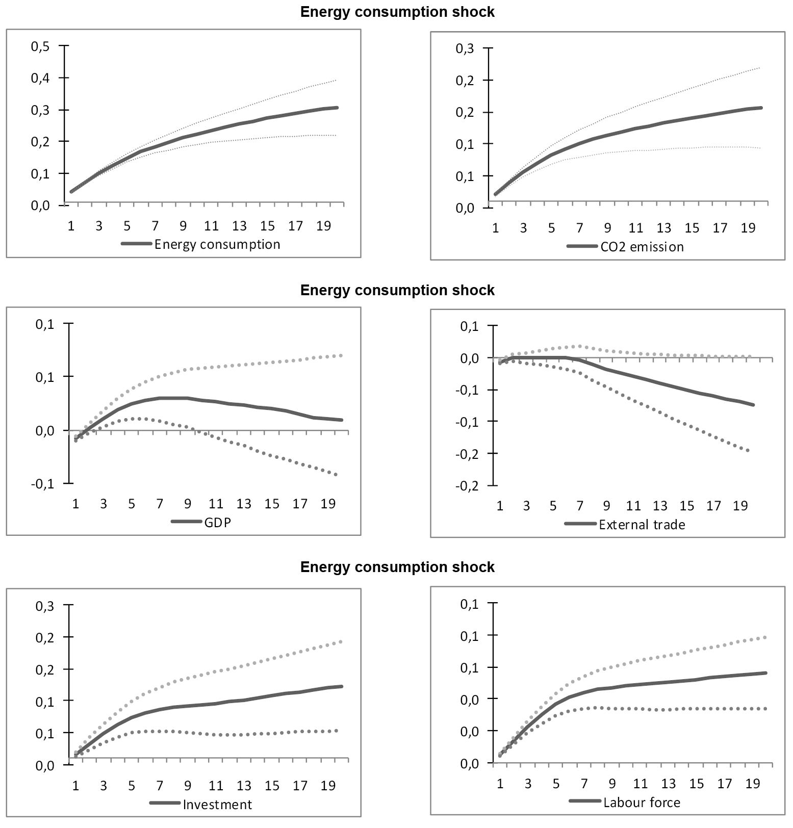
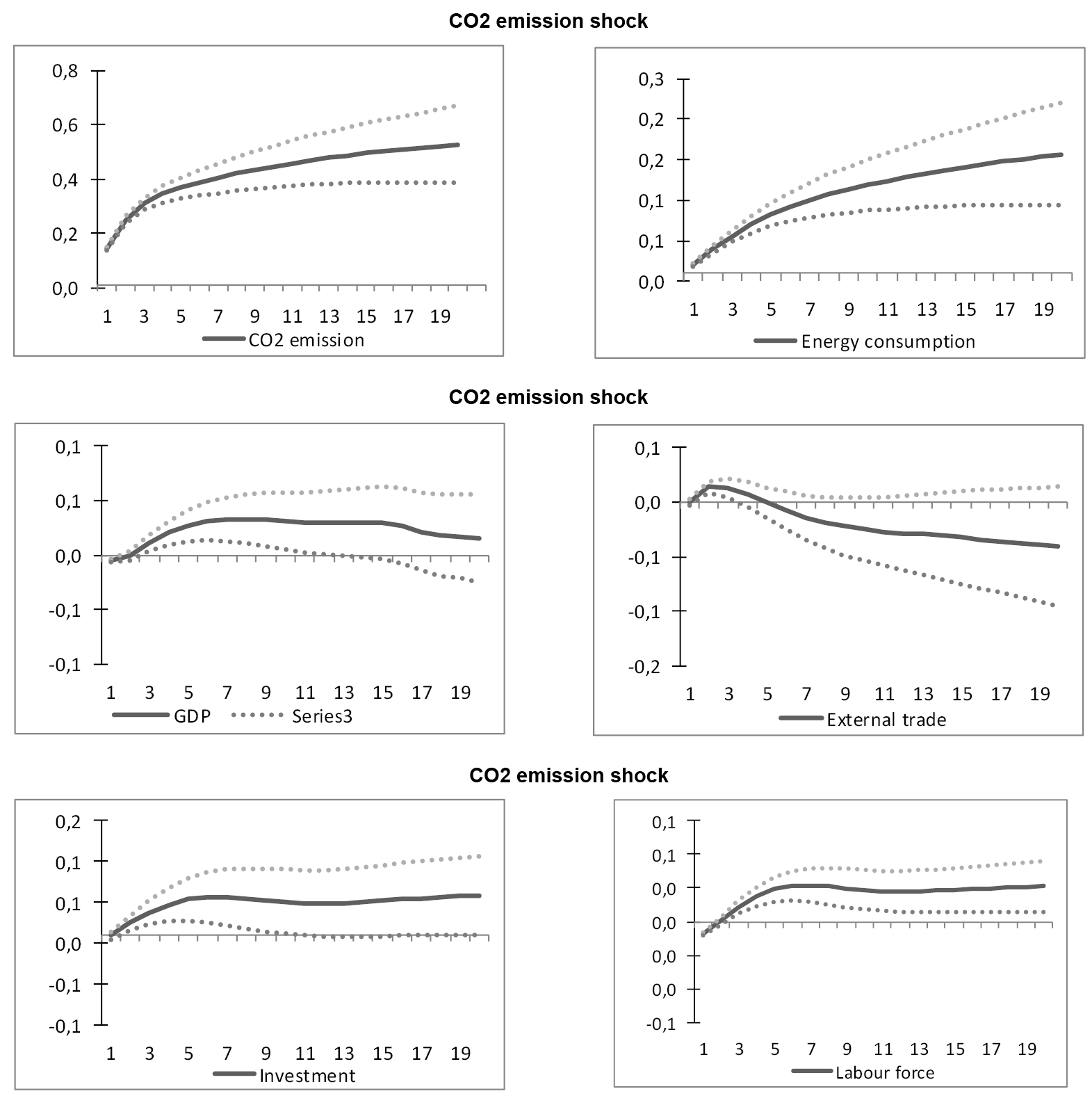
Figure 3. Accumulated generalized impulse response functions for PVAR

Source: Authors’ calculations.

Conclusions

The relationship between climate change mitigation, in our case measured using the reduction of CO2 emissions, greater energy efficiency, and GDP growth is the subject of continuous debate. The economic studies and scientific articles produced to date do not provide a clear answer. Everything depends on datasets used in the analysis, econometric methods applied, and the analyzed countries. In this respect, we cannot yet state that the world has managed to decouple the climate change mitigation and economic growth, i.e., that we have a formula for green economic growth and green transition. All this, though eagerly awaited, is unfortunately yet in the so-called “black box.”

Even theorists tell different stories. According to the Nobel prize winner Nordhaus, CO2 emissions and economic growth are rather contradictory, with an emphasis on the economic growth. However, the main problem is the mainstream neoclassical economic growth theory of the Nobel prizewinning economist Robert Solow, which does not take into account the role of resources in the economy.

In this paper, we have attempted to prove the relationship between economic growth and climate change mitigation while using data for 19 Eurozone countries and applying the PVAR model. The results show that green economic transition is on the right track. GDP depends on energy consumption and CO2 emissions for a very short period and to a small extent.

In our study, we found a short-term negative effect of the environmental policies on economic activity. This is in line with the traditional views that environmental policies might place an additional cost burden on economic activity. However, in the long run, the effects turn positive. As regards economic variables, we found a strong positive effect of the environmental policies on international trade. This confirmed that the most obvious channel through which environmental policies might positively affect economic outcome is competitiveness.

However, empirical evidence showing the effect on investment and employment was inconclusive. The effects of environmental policies on investment might be more complex. Thus, more research would be warranted in this direction. Finally, the analysis presents the usual caveats associated with the use of unrestricted PVAR.

References

Abbas, F., Choudhury, N. (2013). Electricity consumption-economic growth nexus: an aggregated and disaggregated causality analysis in India and Pakistan. Journal of Policy Modeling 35 (4), 538–553, https://doi.org/10.1016/j.jpolmod.2012.09.001

Akinlo, A. E. (2009). Electricity consumption and economic growth in Nigeria: evidence from co-integration and co-feature analysis. Journal of Policy Modeling 31 (5), 681–693, https://doi.org/10.1016/j.jpolmod.2009.03.004

Al-Mulali, U., Saboori, B., Ozturk, I. (2015). Investigating the environmental Kuznets curve hypothesis in Vietnam. Energy Policy 76, 123–131, https://doi.org/10.1016/j.enpol.2014.11.019

Ang, J. B. (2008). Economic development, pollutant emissions and energy consumption in Malaysia. Journal of Policy Modeling 30 (2), 271–278, https://doi.org/10.1016/j.jpolmod.2007.04.010

Antonakakis N., Chatziantoniou I., Filis G. (2017). Energy consumption, CO2 emissions, and economic growth: An ethical dilemma. Renewable and Sustainable Energy Reviews, Volume 68, Part 1, February 2017, Pages 808–824, https://doi.org/10.1016/j.rser.2016.09.105

Apergis, N., Payne, J. E. (2009a). CO2 emissions, energy usage, and output in Central America. Energy Policy 37 (8), 3282–3286, https://doi.org/10.1016/j.enpol.2009.03.048

Apergis, N., Payne, J. E. (2009b). Energy consumption and economic growth in Central America: evidence from a panel co integration and error correction model. Energy Economics 31 (2), 211–216, https://doi.org/10.1016/j.eneco.2008.09.002

Apergis, N., Payne, J. E. (2012). Renewable and non-renewable energy consumption growth nexus: Evidence from a panel error correction model. Energy Economics 34 (3), 733–738, https://doi.org/10.1016/j.eneco.2011.04.007

Apergis, N., Payne, J. E. (2014). Renewable energy, output, Co2 emissions, and fossil fuel prices in Central America: Evidence from a non-linear panel smooth transition vector error correction model. Energy Economics 42 (C), 226–232, https://doi.org/10.1016/j.eneco.2014.01.003

Apergis, N., Payne, J. E., Menyah, K., Wolde-Rufael, Y. (2010). On the causal dynamics between emissions, nuclear energy, renewable energy, and economic growth. Ecological Economics 69 (11), 2255–2260, https://doi.org/10.1016/j.ecolecon.2010.06.014

Arellano, M., Bover, O. (1995). Another look at the instrumental variable estimation of error-components models. Journal of Econometrics 68 (1), 29–51, https://doi.org/10.1016/0304-4076(94)01642-d

Bozoklu, S., Yilanci, V. (2013). Energy consumption and economic growth for selected OECD countries: Further evidence from the Granger causality test in the frequency domain. Energy Policy 63, 877–881, https://doi.org/10.1016/j.enpol.2013.09.037

Caruso G. Colantonio E., Gattone S.A. (2020) Relationships between Renewable Energy Consumption, Social Factors, and Health: A Panel Vector Auto Regression Analysis of a Cluster of 12 EU Countries; Sustainability 2020, 12, 2915, https://doi.org/10.3390/su12072915

Chiou-Wei, S. Z., Chen, C.-F., Zhu, Z. (2008). Economic growth and energy consumption revisited–evidence from linear and nonlinear Granger causality. Energy Economics 30 (6), 3063–3076, https://doi.org/10.1016/j.eneco.2008.02.002

Chontanawat, J., Hunt, L. C., Pierse, R. (2008). Does energy consumption cause economic growth? Evidence from a systematic study of over 100 countries. Journal of Policy Modeling 30 (2), 209–220, https://doi.org/10.1016/j.jpolmod.2006.10.003

Chu, H.-P., Chang, T. (2012). Nuclear energy consumption, oil consumption and economic growth in G–6 countries: Bootstrap panel causality test. Energy Policy 48, 762–769, https://doi.org/10.1016/j.enpol.2012.06.013

Dagher, L., Yacoubian, T. (2012). The causal relationship between energy consumption and economic growth in Lebanon. Energy policy 50, 795–801, https://doi.org/10.1016/j.enpol.2012.08.034

Dasgupta, P., Heal, G. (1974). The Optimal Depletion of Exhaustible Resources. Symposium on the Economics of Exhaustible Resources. The Review of Economic Studies, Vol. 41, pp. 3–28, https://doi.org/10.2307/2296369

Dergiades, T., Martinopoulos, G., Tsoulfidis, L. (2013). Energy consumption and economic growth: Parametric and non–parametric causality testing for the case of Greece. Energy Economics 36, 686–697, https://doi.org/10.1016/j.eneco.2012.11.017

Dinda, S. (2004). Environmental Kuznets curve hypothesis: a survey. Ecological economics 49 (4), 431–455, https://doi.org/10.1016/j.ecolecon.2004.02.011

Donella, H., Meadows, D. L., Meadows, J. R., Behrens, W. (1972). The Limits to Growth. Club of Rome

Eggoh, J. C., Bangak´e, C., Rault, C. (2011). Energy consumption and economic growth revisited in African countries. Energy Policy 39 (11), 7408–7421, https://doi.org/10.1016/j.enpol.2011.09.007

European Commission (2019). Communication “The European Green Deal”, 11 December 2019, in https://ec.europa.eu/info/files/communication-european-green-deal_en

Furuoka, F., (2015). The Co2 emissions–development nexus revisited. Renewable and Sustainable Energy Reviews 51, 1256–1275, https://doi.org/10.1016/j.rser.2015.07.049

Ghosh, S., (2009). Electricity supply, employment and real gdp in India: evidence from co integration and granger-causality tests. Energy Policy 37 (8), 2926–2929, https://doi.org/10.1016/j.enpol.2009.03.022

Grossman, G. M., Krueger, A. B. (1991). Environmental impacts of the North American Free Trade Agreement. Tech. rep., NBER working paper

Halicioglu, F. (2009). An econometric study of co2 emissions, energy consumption, income and foreign trade in Turkey. Energy Policy 37 (3), 1156–1164, https://doi.org/10.1016/j.enpol.2008.11.012

Holtz-Eakin, D., Newey, W., Rosen, H. S. (1988). Estimating vector autoregressions with panel data. Econometrica 56 (6), 1371–1395, https://doi.org/10.2307/1913103

Huang, B.-N., Hwang, M.-J., Yang, C. W. (2008). Causal relationship between energy consumption and GDP growth revisited: a dynamic panel data approach. Ecological economics 67 (1), 41–54, https://doi.org/10.1016/j.ecolecon.2007.11.006

Im, K. S., Pesaran, M. H., Shin, Y. (2003). Testing for unit roots in heterogeneous panels. Journal of Econometrics 115 (1), 53–74, https://doi.org/10.1016/s0304-4076(03)00092-7

Joyeux, R., Ripple, R. D. (2011). Energy consumption and real income: a panel co integration multi-country study. The Energy Journal 32 (2), 107, https://doi.org/10.5547/issn0195-6574-ej-vol32-no2-5

Kijima, M., Nishide, K., Ohyama, A. (2010). Economic models for the environmental Kuznets curve: A survey. Journal of Economic Dynamics and Control 34 (7), 1187–1201, https://doi.org/10.1016/j.jedc.2010.03.010

Kraft, J., Kraft, A. (1978). Relationship between energy and GNP

Levin, A., Lin, C.-F., James Chu, C.-S. (2002). Unit root tests in panel data: asymptotic and finite-sample properties. Journal of Econometrics 108 (1), 1–24, https://doi.org/10.1016/s0304-4076(01)00098-7

Love I., Zicchino L. (2006) Financial development and dynamic investment behavior: Evidence from panel VAR. The Quarterly Review of Economics and Finance, 2006, vol. 46, issue 2, 190–210, https://doi.org/10.1016/j.qref.2005.11.007

M. Allen, Y. Chen, D. Jacob, etc. (2018). Special Report: Global Warming of 1.5 ºC. IPCC, available at https://www.ipcc.ch/sr15

Nordhaus, W.D. (1991). To Slow or Not to Slow: The Economics of the Greenhouse Effect. Economic Journal, Royal Economic Society, vol. 101(407), pages 920–937, https://doi.org/10.2307/2233864

Pesaran, H. H., Shin, Y. (1998). Generalized Impulse Response Analysis in Linear Multivariate Models. Economics Letters 58 (1), 17–29, https://doi.org/10.1016/s0165-1765(97)00214-0

Porter, M. (1991). “America’s Green Strategy”. Scientific American, 264–4

Porter, M. and C. van der Linde (1995). “Toward a New Conception of the Environment-Competitiveness Relationship.” Journal of Economic Perspective, 9–4

R. M. Solow (1974). Intergenerational Equity and Exhaustible Resources. Review of Economic Studies Symposium, pp. 29–46

Robert M. Solow (1956). A Contribution to the Theory of Economic Growth. Quarterly Journal of Economics, volume 70, issue 1, pp 65–94

Sachs, J. (2019), Our zero emissions future. Project Syndicate, 15 April, 2019, at https://www.project-syndicate.org/commentary/zero-emission-energy-and-food-by-middle-of-century-by-jeffrey-d-sachs-2019-04?barrier=accesspaylog

Sachs, J. (2019). Europe’s Green Deal. Project Syndicate, 13 December 2019, at https://www.project-syndicate.org/commentary/europe-green-deal-is-global-beacon-by-jeffrey-d-sachs-2019-12?barrier=accesspaylog

Soytas, U., Sari, R. (2009). Energy consumption, economic growth, and carbon emissions: challenges faced by an EU candidate member. Ecological economics 68 (6), 1667–1675, https://doi.org/10.1016/j.ecolecon.2007.06.014

Stern, D. I. (2004). The rise and fall of the environmental Kuznets curve. World development 32 (8), 1419–1439, https://doi.org/10.1016/j.worlddev.2004.03.004

Stern, D., Cleveland, C. (2004). Energy and economic growth. Working Papers in Economics, Nr. 0410, Rensselaer Polytechnic Institute, USASoytas, U., Sari, R., Ewing, B. T. (2007). Energy consumption, income, and carbon emissions in the United States. Ecological Economics 62 (3), 482–489, https://doi.org/10.1016/j.ecolecon.2006.07.009

Sumskis V., Giedraitis V. (2015) Economic implications of energy security in the short run. Ekonomika 2015 Vol. 94(3), 119–138, https://doi.org/10.15388/ekon.2015.3.8791

Wang, Z., Feng, C. (2015). A performance evaluation of the energy, environmental, and economic efficiency and productivity in China: An application of global data envelopment analysis. Applied Energy 147, 617–626, https://doi.org/10.1016/j.apenergy.2015.01.108

Yıldırım, E., Sukruoglu, D., Aslan, A. (2014). Energy consumption and economic growth in the next 11 countries: The bootstrapped autoregressive metric causality approach. Energy Economics 44, 14–21, https://doi.org/10.1016/j.eneco.2014.03.010

Zhang, B., Wang, Z. (2014). Inter–firm collaborations on carbon emission reduction within industrial chains in China: practices, drivers and effects on firms’ performances. Energy Economics 42, 115–131, https://doi.org/10.1016/j.eneco.2013.12.006

Zhang, X.-P., Cheng, X.-M. (2009). Energy consumption, carbon emissions, and economic growth in China. Ecological Economics 68 (10), 2706–2712, https://doi.org/10.1016/j.ecolecon.2009.05.011

Zhang, Z. (2003). Why did the energy intensity fall in China’s industrial sector in the 1990s? the relative importance of structural change and intensity change. Energy Economics 25 (6), 625–638, https://doi.org/10.1016/s0140-9883(03)00042-2

Annex

Table 1. Panel unit root test results

Variable	Process	Unit root test, p-values
		LLC	IPS	ADF	PP
GDP	Random walk	0,090	0,920	0,930	0,900
	Random walk with intercept and trend	0,951	0,995	0,999	0,991
ΔGDP	Random walk	0,000	0,000	0,000	0,000
	Random walk with intercept and trend	0,000	0,001	0,005	0,000
EC	Random walk	0,825	1,000	0,998	0,762
	Random walk with intercept and trend	0,014	0,433	0,473	0,001
ΔEC	Random walk	0,000	0,000	0,000	0,000
	Random walk with intercept and trend	0,000	0,000	0,000	0,000
CO2	Random walk	0,987	1,000	1,000	0,994
	Random walk with intercept and trend	0,001	0,207	0,085	0,000
ΔCO2	Random walk	0,000	0,000	0,000	0,000
	Random walk with intercept and trend	0,000	0,000	0,000	0,000
LF	Random walk	0,0001	0,0162	0,0252	0,9678
	Random walk with intercept and trend	0,095	0,0579	0,0839	0,9848
ΔLF	Random walk	0,000	0,000	0,000	0,000
	Random walk with intercept and trend	0,000	0,000	0,000	0,000
EXP	Random walk	0,719	1,000	1,000	1,000
	Random walk with intercept	0,001	0,209	0,291	0,754
ΔEXP	Random walk with intercept and trend	0,000	0,000	0,000	0,000
	Random walk	0,000	0,000	0,000	0,000
INV	Random walk with intercept	0,0025	0,0112	0,0248	0,1706
	Random walk with intercept and trend	0,0002	0,04	0,0568	0,2074
ΔINV	Random walk	0,000	0,000	0,000	0,000
	Random walk with intercept	0,000	0,000	0,000	0,000

Note:* represents 5% significance level. The numbers in brackets denote p-values. The LLC test is performed using the Newey-West bandwidth selection with Barlett Kernel, and the Schwartz Bayesian Criterion is used to determine to optimal lag length.

Table 2. Results of lag length selection tests 3 PVAR

Lag	LR	AIC	SC	HQ
1	38,602	-8,011	-5,588	-7,515
2	30,327	-8,108**	-6,787**	-7,605**
3	33,618	-8,231	-6,725	-7,541
4	14,939	-8,232	-6,688	-7,494
5	16,967	-8,249	-6,529	-7,456
6	17,980	-8,275	-6,386	-7,394
7	14,354	-8,279	-6,253	-7,495
8	36,191*	-8,445	-6,097	-7,395

Note: LR (sequential modified Likelihood Ratio test statistic); AIC (Akaike information criterion), SC (Schwarz information criterion); HQ (Hannan-Quinn information criterion); * represents 5% significance level, ** represents the ultimate lag length which was selected for estimation.

Table 3. Results of lag length selection tests 6 PVAR

Lag	LR	AIC	SC	HQ
1	890,219	-15,326	-13,397	-14,547
2	150,715	-15,892	-13,578*	-14,957*
3	52,126	-15,946	-13,247	-14,856
4	39,864	-15,940	-12,855	-14,694
5	24,645	-15,854	-12,383	-14,452
6	65,147*	-16,013*	-12,157	-14,456

Note: LR (sequential modified Likelihood Ratio test statistic); AIC (Akaike information criterion), SC (Schwarz information criterion); HQ (Hannan-Quinn information criterion); * represents 5% significance level, ** represents the ultimate lag length which was selected for estimation.