Ekonomika ISSN 1392-1258 eISSN 2424-6166

2020, vol. 99(1), pp. 110–130 DOI: https://doi.org/10.15388/Ekon.2020.1.7

Exchange Market Pressure and Monetary Policy: The Turkish Case

Ilyas Siklar
Anadolu University, FEAS, Turkey
Email: isiklar@anadolu.edu.tr

Aysegul Akca
Anadolu University, FEAS, Turkey
Email: aysegulsahin@anadolu.edu.tr

Abstract. The purpose of this study is to determine the relationship between monetary policy and the exchange market pressure index in Turkey for the 2002–2018 period with monthly data. To obtain the foreign exchange market pressure index, this study uses the model developed by L. Girton and D.E. Roper and is based fundamentally on the monetary approach to exchange rate determination and the balance of payments. The calculated exchange market pressure index is in accordance with the developments lived in financial markets and changes in monetary policy during the period under investigation. As for the relation between exchange market pressure index and monetary policy, a VAR model was set up and a Granger type causality analysis was carried out. According to Granger causality test results, there is a unidirectional causality running from domestic credit expansion to exchange market pressure and from domestic credit expansion to interest rate differential while there is a bidirectional causality between exchange market pressure and interest rate differential. Since increasing exchange market pressure means a depreciation of the Turkish Lira, the estimated VAR model’s results support the view that the Central Bank will increase the interest rate to temper the exchange market pressure.
Keywords: Exchange market pressure index, Monetary policy, Girton-Roper Model
Received: 16/04/2020. Revised: 07/05/2020. Accepted: 18/05/2020
Copyright © 2020 Ilyas Siklar, Aysegul Akca. Published by Vilnius University Press
This is an Open Access article distributed under the terms of the Creative Commons Attribution Licence, which permits unrestricted use, distribution, and reproduction in any medium, provided the original author and source are credited.

1. Introduction

Developing countries often face problems in the foreign exchange market, so policy choices are important for macroeconomic stability. Domestic economic policies including monetary policies affect the country’s international economic relations. Since the volatility in foreign exchange markets often stimulate unstable foreign trade, consistent monetary regulations are needed to alleviate the pressures arising from foreign exchange markets in developing countries in a globalized world (Weymark, 1998). To determine such pressures, Girton & Roper (1997) define the foreign exchange market pressure as the sum of the depreciation of the nominal exchange rate and the rate of change in international reserves relative to the monetary base. While the monetary approach to the balance of payments is based on a fixed exchange rate, the monetary approach to determining the exchange rate is based on a perfectly elastic exchange rate. However, most countries have neither fixed nor fully flexible exchange rate regimes. In order to overcome these limits set by traditional models, the foreign exchange market pressure criterion, developed by Girton & Roper, can be applied in fixed, fully flexible and managed floating exchange rate systems. Whereas in the fully flexible exchange rate regime the change in international reserves will be zero, the depreciation in domestic currency will be zero under the fixed exchange rate regime. In the managed floating exchange rate regime, the foreign exchange market pressure will be relieved by either the depreciation of the exchange rate, the loss of reserves or a combination of them. Therefore, foreign exchange market pressure can be used as a measure of the magnitude of money market disequilibrium arising from excessive demand or supply in international markets (Klassen & Jager, 2011). Since foreign exchange crises are often defined as periods in which the pressures on the foreign exchange market and the resulting disequilibrium increase sharply, the criterion for foreign exchange market pressure is used to evaluate the effectiveness of monetary policies (Soe & Kakinaka, 2018). This study aims to estimate the extent of exchange market pressure in Turkey for the period 2002–2018 and evaluate the effectiveness of monetary policy. The present study differs from previous ones in the context of applying Girton & Roper Model for the period of inflation targeting monetary policy and floating exchange rate regime. For this purpose, the second section discusses foreign exchange market and monetary policy developments in the corresponding period in Turkey. The third section is devoted to the development of the theoretical model and the review of recent empirical literature. The fourth section aims estimating the model and evaluating the results and, finally, the fifth section concludes the study and provides some policy recommendations.

2. Foreign Exchange Market and Monetary Policy Developments in Turkey

Monetary policy and exchange rate developments are under the influence of economic conditions of the trade partner countries and domestic political changes since the proclamation of the republic in Turkey. The good understanding of the conditions under which the economy operates is a pre-requirement to reveal the targets of economic policies and to determine the necessary tools to reach these targets. In this part of the study, exchange rate and monetary policy developments will be discussed during the review period in Turkey.

One of the most important problems from past to the present has been the high rate of inflation in the Turkish economy. Especially after the 1970s, an economic crisis emerged with an increase in demand inflation and a series of stabilization measures were taken on 24 January 1980. The Turkish Lira was devalued by 32.7%, and a daily exchange rate announcement was applied and aimed to open the economy to foreign markets by liberalizing foreign trade. Banking transactions related to foreign trade were removed from the monopoly of the Central Bank of the Republic of Turkey (CBRT) and transferred to private commercial banks.

The CBRT announced how to proceed in monetary policy in the 1990s. With the announcement of this monetary program, the CBRT foresees to limit the increase in domestic assets and to create TL liabilities as much as the increase in foreign assets. However, in 1993, the political authority announced that the interest burden of the public sector was very high and that policies are needed to reduce interest rates in the short-term. At this stage, a high level of liquidity was injected into the economy; however, contrary to expectation of decreasing interest rates, this excess liquidity began to increase rapidly the demand for foreign exchange.

Changing term structure of the government debt, a high level of the interest rate and the injection of a large amount of money into the economy suddenly affected the exchange rate. While the difference between the market exchange rate and the official exchange rate was 1% in 1993, this difference started to increase at the beginning of 1994. The government, realizing that it could not support any more the value of lira against the increasing demand for foreign exchange, devalued the Turkish Lira in 1994 (Özatay, 2000). At the beginning of 1996, the Central Bank announced its intention to maintain stable real exchange rates and pursued its oversight of exchange rates throughout the year. Interest rates started to decline after reaching the highest level in early 1996 (CBRT, 1996).

After severe earthquake of August 1999, in 2000, Turkey started to implement an IMF-supported stabilization program in which the CBRT announces the nominal exchange rate basket in a regular manner to cover the next 12 months. In June 2000, the general principles of the exchange rate policy and daily upper and lower values of the exchange rate basket to be implemented during July–December 2000 were reported to the markets. Because of speculative attacks and a fragile banking system, interest rates skyrocketed to 3000% while the CBRT tried to defend the Turkish Lira at the end of 2000. The results were heavy losses in international reserves and the collapse of the financial system as a whole. Together with the IMF, it was decided that it is impossible to implement the current exchange rate policy because of the heavy burden on the economy. Turkey started to implement a new pragmatic stabilization program (Program of Transition to a Strong Economy) in February 2001, in which the value of the Turkish Lira was left to fluctuate within the band against foreign currencies. The main idea in these exchange rate regime and economic policy changes was that exchange rate would not be used any more as a monetary policy tool.

The CBRT announced in 2002 that the ultimate goal of monetary policy was to switch to inflation targeting. The 2002–2005 period was declared as a preparatory period in which the necessary steps would be taken to eliminate the factors limiting the effectiveness of the monetary policy in order to achieve this ultimate goal. Two types of nominal anchors were identified in 2002 to reduce forward-looking uncertainties and to shape expectations: monetary targeting and inflation targeting. Monetary policy in 2002 started with monetary targeting and aimed to implement a monetary policy focusing on “future inflation”. A monetary policy focusing on “future inflation” also means “implicit inflation targeting” (CBRT, 2002: 7). Besides, to shape the inflationary expectations, the purposes of implicit inflation targeting policy were to control factors determining costs and affecting domestic aggregate demand in order to reduce inflationary pressures. Therefore, the year 2002 was accepted as the beginning of a three-year transition to a strong economy. The targeted monetary aggregate was the monetary base and the target was an increase in monetary base as much as nominal GDP growth in 2002. Desired results in monetary base as intermediate target and in net international reserves and net domestic assets as operating targets (these are called as performance criteria in the Program) were obtained during this period (Sarı, 2007: 16). As a result of converging inflation rate closer to target, CBRT introduced six interest rate cuts between 2002 and 2005. During the five-year period until 2006, compliance with the floating exchange rate regime has increased and significant progress has been made to create a favorable environment for the transition to inflation targeting regime: all inflation targets have been achieved, reliability has increased and inflation expectations have converged to the targets. The inflation rate has reached its lowest level in the last thirty years. Concerns about the sustainability of fiscal discipline have largely decreased. The depth of financial markets began to increase and the fragility of the financial sector decreased (CBRT, 2006: 1). These developments indicate that the pre-requirements for transition to explicit inflation targeting in 2006 were met.

Inflation-targeting central banks announce their targets to people, promise to reach these targets and are responsible to account for in case of failing to catch up these targets. As monetary policy decisions require some certain time to affect the economy, central banks can control the future inflation rather than the current one. For this purpose, they estimate the inflation rate for certain periods and share these estimates with the public (CBRT, 2006: 3). Upper or lower deviations of the realized inflation from the target are equivalently evaluated in inflation targeting monetary policy regime. The fact that the actual inflation remains below the target is as important as being above the target, and the reasons should be disclosed to the public. “Inflation Report” and “Monetary Policy Committee Report” that CBRT publishes in the context of inflation targeting are used as main communication tools. With the introduction of inflation targeting regime, the Monetary Policy Committee (MPC) continued to convene on a monthly basis in accordance with a predetermined and publicly announced calendar. Decisions regarding interest rates have been taken by voting at the MPC meetings and announced on the same day with their justifications. In other words, in monetary policy decisions, the MPC has changed from a referring position to a decision-making position.

In 2006, CBRT announced that it has no target for the exchange rate and it is solely determined by the supply and demand factors in the market while the essential determinants of the exchange rate are the monetary and fiscal policies. Deteriorations in economic fundamentals, developments regarding the stabilization program and expectations may cause to fluctuate exchange rates in the economy. Since 2002, CBRT’s intervention in exchange rates has generally been through foreign exchange buying auctions.

Toward the end of 2008, increasing volatility and loss of confidence in the global financial markets increased the demand for the US dollar and caused a significant depreciation of TL. During these periods, CBRT used its reserves to support the foreign exchange liquidity of the banking system. During the crisis period, it interrupted foreign exchange buying auctions and tried to meet the foreign exchange liquidity needs of the market through selling auctions. With the intensification of the global financial crisis, interest rates were cut to ease the tightening in the market.

The main policy instrument of the CBRT is short-term interest rates. However, one of the lessons learned from the 2008 crisis is that other monetary policy instruments may need to be used to reduce macroeconomic risks, especially during periods of overheating of the economy. In this context, due to future developments, for example, if the rate of expansion in loans exceeds the desired levels, required reserve ratios can be used more actively as a policy instrument to reduce macroeconomic risks (CBRT, 2010: 12)

Since the end of 2010, apart from traditional practices to limit the negative effects of the crisis, CBRT has designed a new monetary policy which can react to shocks. For this purpose, the inflation targeting regime, which has been implemented since 2006, has been developed in a manner to ensure financial stability. In this revision, CBRT aimed to temper the current inflation targeting regime with an active liquidity policy in which an asymmetric and wide corridor system with multiple interest rates is used. In this period, the CBRT has also diversified its policy instruments like reserve option mechanism and corridor system. By doing so the CBRT has taken steps to ensure financial stability without compromising price stability (CBRT, 2017).

Figure 1 and Figure 2 show the course of the exchange rates and interest rate during the review period, while Table 1 indicates key macroeconomic indicators for the last ten years. When the figures are examined, although a certain level of stability has been achieved in interest rates, it is not possible to say the same for the exchange rate.

Figure 1. USD/TR and EURO/TR Exchange Rates for 2001–2018 Period

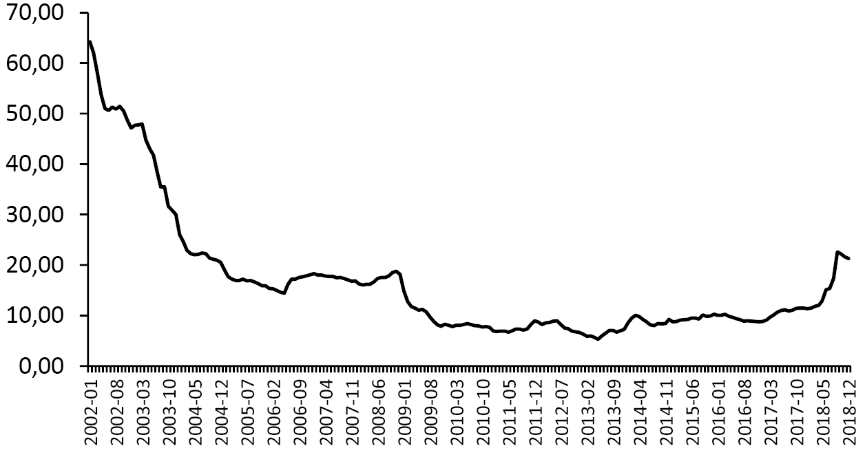
Figure 2. Short Term Interest Rate for 2001–2018 Period

Table 1. Fundamental Macroeconomic Indicators (2009–2018)

Indicator	2009	2010	2011	2012	2013	2014	2015	2016	2017	2018
GDP Growth Rate (%)	-4.8	9.2	8.8	2.1	4.2	3.0	6.1	3.2	7.5	2.8
CPI Inflation (annual - %)	10.1	6.5	10.5	6.2	7.4	8.2	8.8	8.5	11.9	20.3
Unemployment Rate (%)	14.0	11.9	8.5	8.8	9.1	10.4	10.2	12.0	9.9	12.9
Import Coverage Ratio (%)	72.5	61.4	56.0	64.5	60.3	65.1	69.4	71.8	67.1	75.3
Current Acc. Balance/GDP (%)	-2.0	-6.2	-9.6	-6.1	-7.7	-5.5	-3.2	-3.1	-4.8	-2.6
Budget Balance/GDP (%)	-5.5	-3.6	-1.4	-2.1	-1.2	-1.3	-1.0	-1.1	-1.5	-1.9
Total Debt Stock/GDP (%)	44.2	40.8	37.2	33.9	32.4	30.0	29.0	29.1	28.2	28.7

Source: The Central Bank of the Republic of Turkey, Electronic Data Delivery System.

Following the 2008 crisis, it became more difficult for central banks to follow developments and regulations in the financial markets. Therefore, central banks have focused on the development and calculation of financial pressure indices and exchange rate pressure indices. Girton & Roper (1977), who made the first study on foreign exchange market pressure, defined the foreign exchange market pressure as “the magnitude of the intervention to be made in order to reach the desired exchange rate level”. In the following sections of the study, first the theoretical background and literature are presented; then, background information is given about Girton & Roper model and finally the estimation method and results are explained.

3. Measurement of exchange market pressure

In this section, we will first review the theoretical models of measurement of foreign exchange market pressure and the recent literature on these models and then develop Girton & Roper model by obtaining the necessary equations to be estimated in this study.

3.1. Theoretical Background and Recent Literature

Most of the studies aimed at measuring the pressure of the foreign exchange market on the economy use one of the four basic methods, which may be dependent on or independent of a structural macroeconomic model. These four methods can be listed as follows: (1) Girton & Roper (1977) Model, (2) Roper & Turnovsky (1980) Model, (3) Eichengreen, Rose and Wyplosz (1995, 1996) Model and (4) Weymark (1985) Model. It is generally accepted that Roper-Turnovsky and Weymark Models are model dependent while Girton-Roper and Eichengreen-Rose-Wyplosz Models are model independent.

Girton & Roper (1977) use the asset market approach to the balance of payments to address the excess currency demand within the framework of a two-country small open economy model and, on the basis of this, calculate the foreign exchange market pressure for Canada. In the model, the Central Bank’s decisions regarding domestic credit expansion are exogenous and only changes in foreign exchange reserves and exchange rates can alter the foreign exchange market pressure. In this approach, the changes observed in foreign exchange reserves and exchange rates are included in the model with an equal weight. Accordingly, foreign exchange market pressure (EMP) in period t is defined as:

(1)

In this equation Δet refers to percentage change in the exchange rate, while Δrt stands for the percentage change in foreign exchange reserves of the central bank. Since Δet = 0 in a fixed exchange rate regime, EMPt = Δrt. However, since Δrt = 0 in a flexible exchange rate regime, EMPt = Δet. Here, the EMP measure is obtained depending on the model, but this method is evaluated as model-independent, since both terms in Equation (1) have equal weights.

The method developed by Roper & Turnovsky (1980) uses a stochastic small economy IS-LM model to measure the excessive demand for domestic currency. In this model, it is assumed that the excess demand for domestic currency is absorbed by not only changes in exchange rate and foreign exchange reserves but also changes in domestic credit volume.

(2)

In addition to already defined variables, Δdt and η refers to change in domestic credit volume and exchange rate elasticity of domestic credit (with a negative sign). The value of this elasticity is obtained through a structural model of the economy. In the Roper & Turnovsky Model, the calculation of EMP requires estimation of some parameters: (1) Interest rate elasticity of output, (2) Output and interest rate elasticities of monetary base and (3) Exchange rate elasticity of interest rate.

Eichengreen, Rose and Wyplosz (1995) claim that model dependency is not a desirable feature for EMP index. They insist that structural models have a considerable weak explanatory power for medium term forecasting. Since central banks use interest rate increases against speculative attacks, EMP index should include the interest rate differential. Therefore, this model involves percentage change in interest rate differential channel in addition to channels of Girton & Roper Model (percentage changes in exchange rate and foreign exchange reserves) in the construction of exchange market pressure. Sine each component of the EMP index is weighted considering its sample variance, there is no need to estimate a structural model representing the economy. If we denote the interest rate differential between domestic and foreign interest rates with (i – i*), exchange market pressure is calculated as:

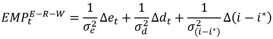(3)

Weymark (1988) claims that the models developed by Girton & Roper (1977) and Girton & Turnovsky (1980) have not made adequate effort to derive the exchange market pressure conceptually. In the Girton & Roper (1977) study, EMP is derived to determine the magnitude of exchange market intervention in order to reach the desired exchange rate target. In the Girton & Turnovsky (1980) study, on the other hand, optimal stabilization policy in a small open economy is emphasized. For a small open economy, Weymark (1998) obtains the model dependent exchange market pressure as:

(4)

Here, Δft is the percentage change in foreign exchange reserves and η is the reserve elasticity of foreign exchange rate. To estimate coefficient η, there are two parameters that should be obtained in the structural model of the economy: (1) the exchange rate elasticity of the domestic price level and (2) the domestic interest rate elasticity of money demand. Weymar (1998) claims that EMPG-R ve EMPG-T measures are the special cases of this indicator. However, Weymark (1998) model drives out sterilization possibilities in the foreign exchange market interventions of the central bank.

It has been seen during the last two decades in the literature that conclusions regarding to relationship between EMP and monetary policy are conflicting. Tanner (2001) analyzes whether monetary policy affected EMP in Brazil, Chile, Mexico, Indonesia, South Korea and Thailand during 1990s and seeks evidence for the proposition that tight monetary policy reduces EMP. In that study, EMP is estimated for individual countries and the whole countries by using credit expansion and interest rate differential variables. Results show that reductions in domestic credit volume decrease EMP for both individual and overall countries. While for some countries, a positive interest rate shock reduces EMP, it is determined that EMP shocks positively affect interest rates on the basis of individual and all countries.

By using the EMP concept, Jeisman (2005) investigates the effects of foreign exchange interventions of the Reserve Bank of Australia on exchange rate. The obtained results show that the Reserve Bank’s interventions have more power when the exchange rate depreciates.

In the study carried out for Philippines, Bautista & Bautista (2005) tries to evaluate the reaction of monetary authority to EMP changes using the VAR methodology. Conclusions of this study differ for crisis and non-crisis periods. While the monetary authority tends to sterilize the effects of the EMP in non-crisis periods, it does not go to sterilization in times of crisis and tends to slow down domestic credit expansion.

In the study conducted by Garcia & Malet (2007) for the Argentinean economy, the interaction between EMP and monetary policy is examined by considering economic growth. According to the results obtained by the VAR methodology, an increase in the domestic interest rate does not cause a decrease in EMP, while an increase in the US interest rate affects EMP. On the other hand, since economic growth in Argentina is largely dependent on foreign capital inflows, the impact of growth on EMP is found to be stronger than the impact of domestic credit volume or interest rate. In another similar study involving Estonia, Latvia, Lithuania and Bulgaria, Hegerty (2009) obtained the same results for the fixed exchange rate regime. Intense capital inflows increase the devaluation pressure and may adversely affect economic growth.

In a study by Hall et al. (2013), the time-varying weights version of the Girton & Roper model is used for EMP estimation. According to estimates made on the basis of Yen, Yuan, Pound and Dollar, EMP shows that Yen and Yuan are overvalued against the Dollar, while the Pound is a free-floating currency.

Ahmed (2013), based on the Pakistani economy, examines the foreign exchange market imbalances through the VAR model. According to the results, while the foreign exchange market is the main reason of the disequilibrium in the domestic money market, the efforts of the monetary authority to reduce the exchange rate pressure through money supply are not effective. The reason for such a situation is that sterilization has no effect when increasing domestic credit volume reduces international reserves.

3.2. The Girton & Roper Model

When obtaining the exchange market pressure measure, the Girton & Roper (1977) study uses models related to monetary approach to balance of payments and exchange rate determination. The developed model is based on the domestic and foreign monetary sector conditions and consists of the following equations:

(5)

(6)

(7)

(8)

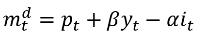
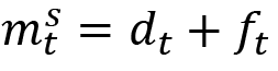
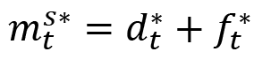
Equation (5) is the demand for money function and indicates that money demand (md) is positively related with income (y) and negatively related with interest rate (i). Equation (6) is the money supply (ms) equation and indicates that the total of domestic credit volume (d) and international reserves (f) constitutes the supply of money. Lower case letters in above equations show logarithmic values while star superscript indicate foreign counterparts of the domestically defined variables. Money market equilibrium means equality of demand for and supply of money:

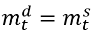(9)

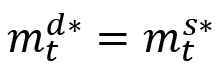(10)

If we consider the first difference form of domestic and foreign money markets equilibrium, we get

(11)

(12)

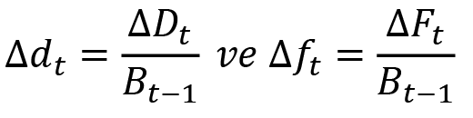
Girton & Roper (1977) define the rate of change in domestic credit volume and international reserves as:

If we subtract foreign money market equilibrium (12) from the domestic money market equilibrium (11) and rearrange, we have

(13)

Under the assumption that relative purchasing parity condition holds:

(14)

Here, Δe and Δq stand for the percentage change in nominal and real exchange rates, respectively. In the last equation, the foreign exchange rate is defined as the value of one unit of foreign currency in terms of domestic currency. Thus, an increase in Δe means a depreciation in domestic currency. Rearranging (14) gives

(15)

If we put (15) in (13) and rearrange the product, we get

(16)

If purchasing power parity holds, Δqt drops from the equation. According to Girton & Roper (1977), deviations from purchasing power parity (Δqt) can be accepted as a linear function of expansions in domestic credit volume and foreign money supply:

(17)

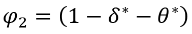
In the last equation stating deviations from purchasing power parity it is expected that θ>0 ve θ*>0. If we substitute the last equation in (16), which explains the changes in nominal exchange rate and rearrange, we get

(18)

It should be noted that, unlike the previous equations, rates of domestic credit expansion and foreign monetary expansion have coefficients different from -1. Since parameter θ is not related with the monetary expansion arising from international reserve changes, the coefficient of Δft (change in international reserves) equals -1 as before. Therefore, the last equation can be rewritten as:

(19)

On the left hand side of the last equation, the total of change rates of nominal exchange rate and international reserves (Δet + Δft) measures exchange market pressure without estimating any structural macroeconomic model. If we accept the validity of full capital mobility, we will have

(20)

This equation is the interest rate parity condition and states that differential between domestic and foreign interest rates will be reflected to the expected exchange rate. Substituting (20) in (19) and rearranging yields

(21)

If we define,

by rewriting (21), we can obtain the exchange market pressure equation that is used by Girton & Roper (1977) as:

(22)

In this equation, ξt is the error term with traditional properties. Equation (22) is the fundamental equation used in our study to estimate exchange market pressure indices.

4. Estimation methodology and results

In the Girton & Roper (1977) model, exchange market pressure index is obtained from the flexible price monetary equilibrium model developed by Frenkel (1976). This model given in (22) will be estimated as follows with the addition of the interest rate differential variable (it –i*t ) in order to evaluate the relationship between monetary policy and exchange market pressure:

(23)

4.1. Estimation Period and Data

Almost 70% of Turkey’s foreign trade is with European countries. Contrary to previous studies, this study measures the foreign exchange rate as TR/Euro parity and, naturally, variables with “foreign country” origin will be represented with European Union Region data.

Turkey is a country that has carried out radical changes in its monetary policy and foreign exchange regime after the 2001 financial turmoil as we discussed earlier. In order to exclude the structural breaks caused by the financial crisis and policy transformation, the estimation period will be initiated from 2002. In addition, it will be preferred to use monthly data to see the dynamic structure presented by the model more clearly. Therefore, the estimation period starts with January 2002 and ends with December 2018. Since it is not possible to find the data on monthly basis for domestic and foreign outputs (y ve y*), we prefer to use manufacturing industry production index as proxy variables. The time series data for the domestic variables and foreign variables are obtained from CBRT’s electronic database and Eurostat, respectively. Figure 3 depicts the course of the time series during the estimation period, while Table 2 summarizes the statistical properties of the time series used in the study.

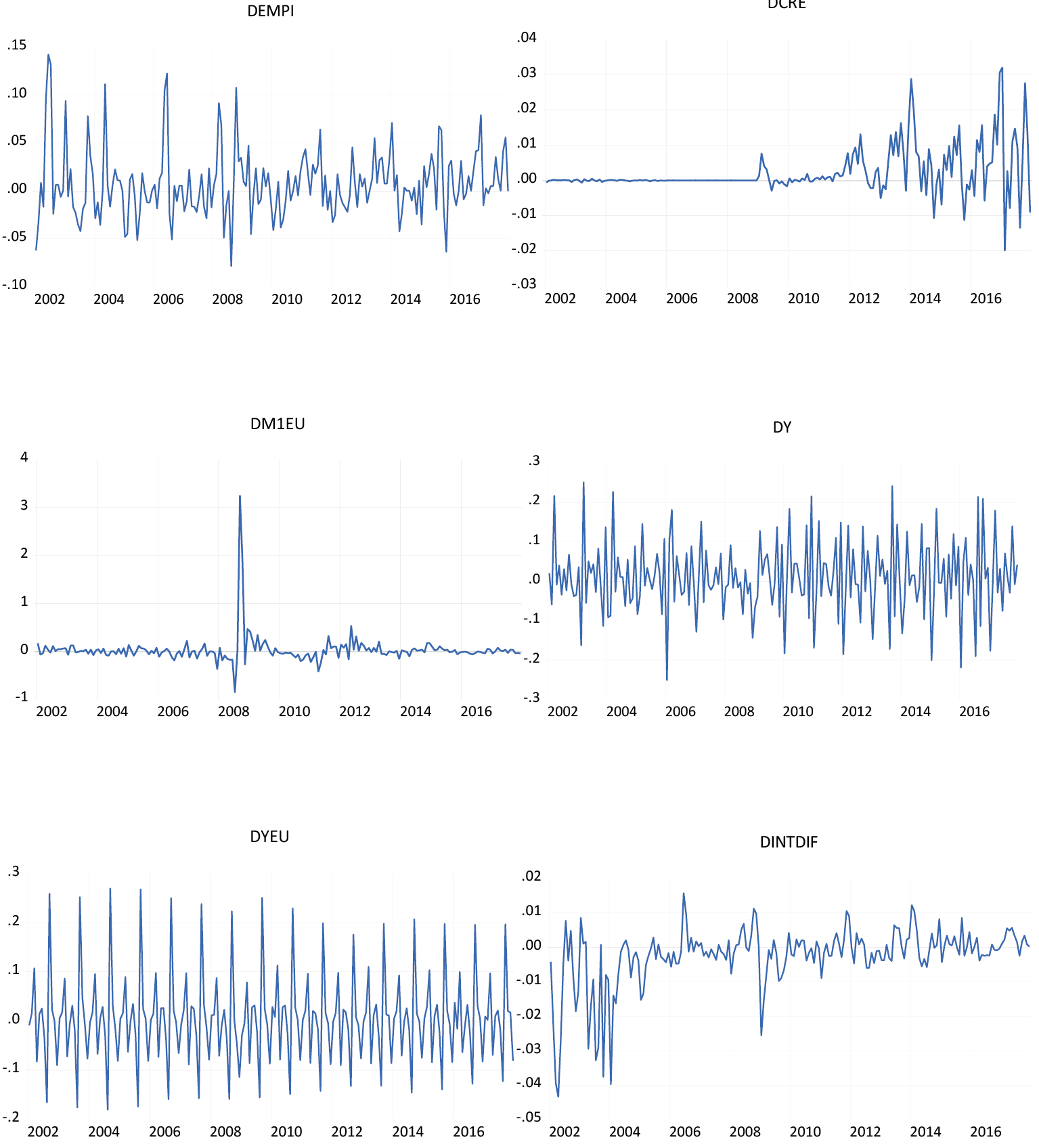
Figure 3. Time Series Plot of the Variables during Analyzing Period

Table 2. Time Series Properties of Variables

	DEMPI	DCRE	DM1EU	DY	DYEU	DINTDIF
Mean	0.007228	0.002179	0.028042	0.010310	0.004704	-0.002578
Median	0.003592	9.57E-06	0.000500	-9.90E-05	0.004450	-0.001200
Maximum	0.142106	0.032023	3.246000	0.250840	0.269762	0.015700
Minimum	-0.078573	-0.019845	-0.853000	-0.250668	-0.180884	-0.043400
Std. Dev.	0.035454	0.006587	0.301142	0.092970	0.091697	0.008934
Skewness	1.115128	1.707556	7.474150	0.080322	0.755127	-2.177942
Kurtosis	5.279440	9.007499	76.46342	3.279273	4.130699	9.408404
Jarque-Bera	81.35910	382.0243	44962.60	0.830396	28.47477	480.3309
Probability	0.000000	0.000000	0.000000	0.660210	0.000001	0.000000
Sum	1.387772	0.418436	5.384000	1.979560	0.903242	-0.495000
Sum Sq. Dev.	0.240090	0.008287	17.32110	1.650900	1.605981	0.015244
Observations	204	204	204	204	204	204

4.2. Estimation Methodology and Results

The ordinary least squares method is used by Girton & Roper (1977) to analyze factors affecting exchange market pressure index (EMPI). However, ordinary least square is not the proper estimator, since the existing feedback among variables (particularly between domestic credit expansion and EMPI, interest rate differential and exchange rate-therefore EMPI-) causes an endogeneity problem (Bielecki, 2005; Younus, 2005). Therefore, in order to investigate the interaction between monetary policy and EMPI, this study uses VAR methodology in which the endogeneity problem among variables are completely solved. On the other hand, through impulse-response functions, this methodology gives the opportunity to see how shocks in endogenous variables affect the other variables in the model. Since the number of observations will be sufficient due to the use of monthly data, the small sample problem will be overcome.

Assuming that Turkey is a small open economy, the change rate of foreign money supply and the change rate of foreign output in equation (23) above are accepted as exogenous variables. Accordingly, the VAR model to be estimated takes the following form:

(24)

where y' is the vector of endogenous variables and x' is the vector of exogenous variables (and ), while ω' is the vector of error terms. According to unit root tests with structural breaks, all the variables are integrated of order one [i.e. I(1)] and there is no cointegration relationship among variables (see Appendix 1 for results of both tests), indicating VAR is the proper estimator for equation (24). Considering the various lag selection criteria, the optimal lag length is chosen as 1 month in the estimation of the VAR model (see Appendix 2). Table 3 summarizes the estimation results of the VAR model and the related test statistics.

Table 3. Estimation Results of VAR Model

Variable	Δy	t†	Δd	t	Δ(i-i*)	t	Δe+Δf	t
Δyt-1	-0.40	6.21*	-0.01	0.43	-0.01	2.14*	-0.03	1.04
Δdt-1	0.82	0.87	0.33	4.51*	0.05	0.59	0.70	1.85**
Δ(i-i*)t-1	-0.04	0.06	0.06	1.20**	0.53	8.66*	-0.70	2.53**
Δet-1+Δft-1	-0.25	1.42**	-0.01	0.97	0.04	2.46*	0.31	4.42*
AdjR2	0.26	--	0.12	--	0.35	--	0.15	--
F	10.62*	--	4.01*	--	16.68*	--	5.33*	--

† shows the absolute t-statistic value for the relevant coefficient

*, ** and *** indicate the statistical significance of the estimation at 1, 5 and 10 percentage levels, respectively.

According to Table 3, the coefficients for the domestic credit expansion and interest rate differential in the foreign exchange market pressure equation have expected signs and are statistically significant. Low explanatory power of the equation seems natural and emphasizes the fact that CBRT focuses on the inflation rate rather than credit volume or exchange rate in the inflation targeting regime. In the domestic credit expansion equation, the coefficient of exchange market pressure is close to zero, and that can be accepted as an indication of insufficient sterilization during the analyzed period. On the other hand, this explains the positive credit expansion coefficient in the exchange market pressure equation. A similar case also applies to interest rate differential equation. Positive and statistically significant coefficient of exchange market pressure exhibits the importance of interest rate differential in foreign exchange market. When we consider Table 3 as a whole it is possible to say that we have specifically correct but statistically weak VAR system because of low explanatory power. This should be regarded as a normal outcome under the monetary policy regime towards inflation targeting. However, a statistically significant interest rate differential and exchange market pressure in related equations indicate the existence of a powerful interaction between these variables.

Because of the fact that VAR models are atheoric in their nature, it requires to analyze the direction of interactions among variables before analyzing the validity of these interactions. To avoid possible bias, we conducted causality tests with one-month lag as determined in the lag order selection of the VAR model (See Table A3 in the appendix). Granger causality test results that are generally used for this purpose are presented in Table 4.

Causality tests produce two interesting findings in terms of the subject we are studying. First of all, there is no causal relationship between domestic credit expansion and foreign exchange market pressure, domestic credit expansion and interest rate difference. While this result is consistent with VAR model in terms of interest rate differential, it is contradictory with VAR model in terms of exchange market pressure. The fact that the interest rate differential does not have a significant effect in VAR model and produces a result of accepting the causality relationship indicates that the Central Bank is away from sterilization. This is also an indication of the fact that, in monetary policy formulation, the Central Bank considers the estimated inflation rather than inflation target. While a statistically significant relationship between domestic credit expansion and exchange market pressure in the VAR model is obtained, rejecting the causality relationship between the same variables stems from the lag structure of the model. To avoid any possible bias, causality tests are performed with the same lag length of the VAR estimation (1 month). However, if we increase the lag length to two months, there exists a unidirectional causality from exchange market pressure to domestic credit expansion in the 5% level of significance, while increasing the lag length to three months produces bidirectional causality between them at 1% level of significance. The second interesting result produced by causality tests in accordance with the VAR model is the bidirectional causality relationship between exchange market pressure and interest rate differential. The result obtained from the VAR model indicate that the international interest rate parity condition holds while the bidirectional causality relationship shows that the domestic interest rate is kept under pressure. Findings indicating a significant effect of exchange market pressure on domestic credit expansion and the non-rejection of this relationship in causality tests strengthen this view.

Table 4. Results of Granger Causality Tests

Null Hypothesis	Lag Length	F Statistic	Probability	Conclusion
Δy does not cause Δd Δd does not cause Δy	1 1	0.18 1.48	0.67 023	No causality relationship
Δy does not cause Δ(i-i*) Δ(i-i*) does not cause Δy	1 1	4.78 0.46	0.03 0.50	y → (i-i*)
Δy does not cause (Δe+ Δf) (Δe+ Δf) does not cause Δy	1 1	1.86 3.04	0.17 0.08	(e+f) → y
Δd does not cause Δ(i-i*) Δ(i-i*) does not cause Δd	1 1	1.05 1.13	0.31 0.29	No causality relationship
Δd does not cause (Δe+ Δf) (Δe+ Δf) does not cause Δd	1 1	2.09 0.68	0.15 0.41	No causality relationship
Δ(i-i*) does not cause (Δe+ Δf) (Δe+ Δf) does not cause Δ(i-i*)	1 1	5.31 5.07	0.02 0.03	(i-i*) ↔ (e+f)

The impulse-response functions that make sense in terms of the subject we have discussed can be examined by considering Figure 4 below. Although some of the confidence intervals puts suspicion toward statistical validity of responses (like panel B, C and F), they should be accepted as general indication of the changes in the model since the estimated VAR model equations are statistically significant (see Table 3). In panel A of the figure, the response of exchange market pressure to a shock in the domestic credit volume is given, while panel B shows the response of domestic credit volume to a shock in exchange market pressure. The foreign exchange market pressure simultaneously and positively reacts to the domestic credit shock and this reaction proceeds in a gradually declining manner throughout six months. This supports the traditional theoretical expectation that domestic currency appreciates and international reserve volume increases if the Central Bank engages foreign currency purchasing transactions to draw the excess liquidity in the market (or vice versa; domestic currency depreciates and international reserves decline if there are foreign exchange selling operations). According to panel B of the figure, domestic credit volume responds with a substantial lag to a shock in exchange market pressure. This is evidence proving that the value of domestic currency should be defended in order to restrict the expansion in domestic credit volume in the economy. However, if we consider the fact that this response is short lived and limited, we can say that measures that aim to defend the value of domestic currency should contain small scaled and temporal interventions without creating fundamental changes in international reserves.

Panel C and D of Figure 4 shows effects of interest rate differential shock on exchange market pressure and effects of exchange market pressure shock on interest rate differential, respectively. In line with theoretical expectations, a positive shock in interest rate differential increases the foreign exchange market pressure through the depreciation of the domestic currency. This effect gradually diminishes and blows out in 6 months and supports the results obtained with causality tests. In panel D, which presents the effects of a shock in exchange market pressure on interest rate differential, it is seen that depreciation of domestic currency (or reductions in international reserves) forces Central Bank to increase interest rate in order to reduce the increasing pressure. Otherwise we can say that participants of exchange market demand greater risk premium. Since this effect is short lived and relatively small, the Central Bank gives strong signals to the markets indicating it has no predetermined target for exchange rate and its main interest is the price stability (this signal can also be evaluated as “it will avoid exchange market interventions”).

Panel E of Figure 4 presents the effects of a shock in domestic credit volume on interest rate differential, while Panel F shows vice versa. According to Panel E, a positive domestic credit shock creates a simultaneous increase in interest rate differential. Considering the incomplete exchange rate pass-through findings of the previous studies (see, for instance, Siklar et al., 2017; Siklar-Uslu, 2007; Arslaner et al., 2014), this result is rather surprising. One possible reason for this situation is the high inflationary expectations stemming from unreached inflation targets throughout analyzing period. Despite this relationship, according to the F panel of the figure, the response of the domestic credit volume to the interest rate differential shock remains quite weak. This is consistent with the Granger type causality tests discussed earlier in this study. This weak response also supports the findings of the incomplete interest rate pass-through (see for instance, Binici et al., 2016; Yıldırım, 2013; Siklar et al., 2016).

By applying a similar model and estimation technique, Garcia & Malef (2005) for Argentina, Ziramba (2007) for South Africa and Ratnasari & Widodo (2017) for ASEAN5 (Indonesia, Malaysia, the Philippines, Thailand, and Singapore) obtain parallel results for output and credit growth. One interesting point is that although the mentioned papers use different variables (especially the US-based foreign variables) and cover different time periods that correspond different monetary policy and exchange rate regimes, they reach almost the same conclusion on interest rate differential and capital flows like us. This indicates the importance of the existence of currency substitution and high inflation history in the estimation of exchange market pressure in the economy. Although it uses a different model but the same estimation technique to analyze the relationship between exchange market pressure and domestic credit growth in Poland, Bielecki (2005) reaches the same conclusion as us: the sterilization of the reserve flows is the key factor for exchange market pressure besides official foreign exchange interventions and other currency market operations with commercial banks.

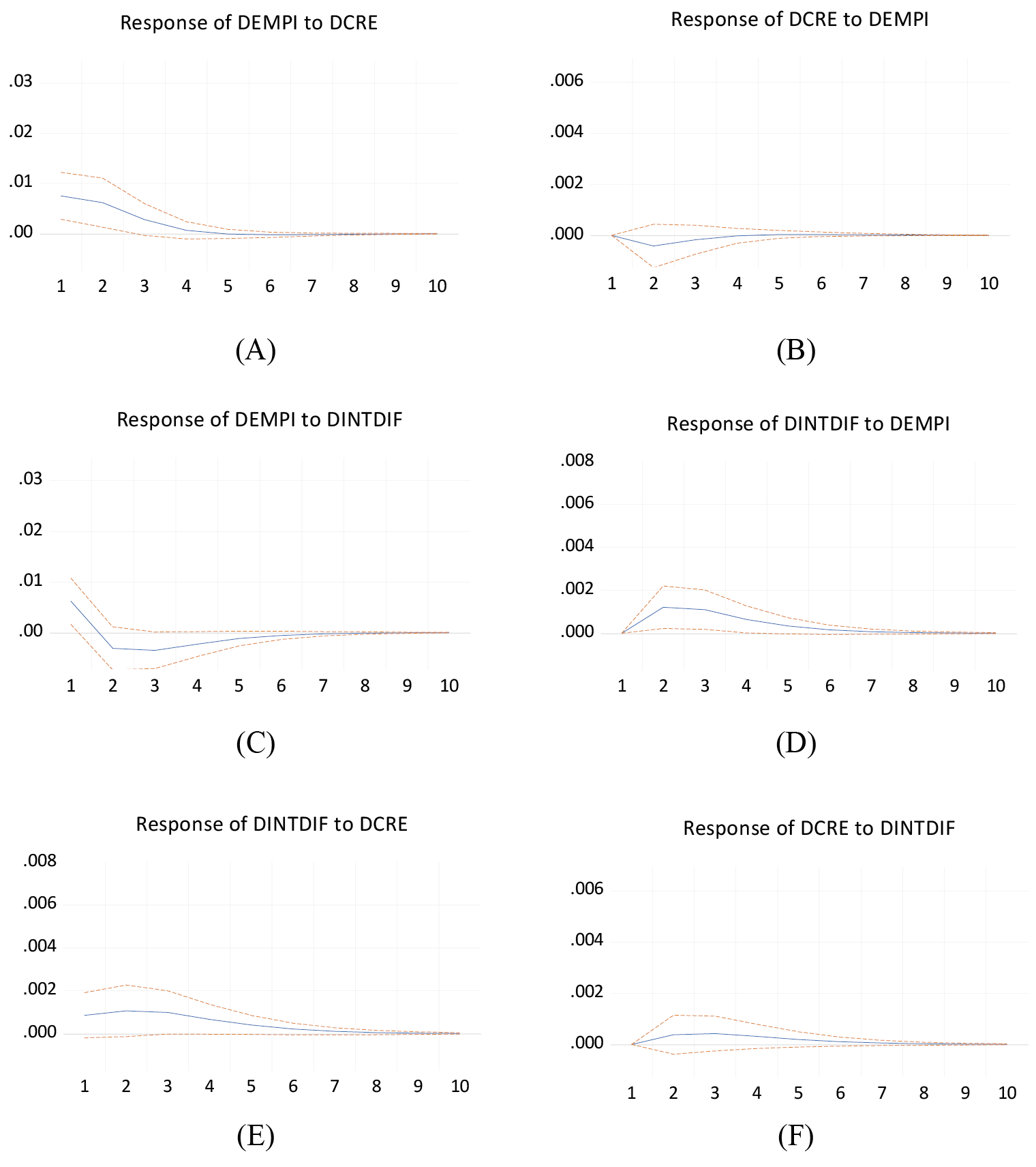
Figure 4. Impulse – Response Functions

Analyzing MENA Region countries (Turkey, Egypt and Tunisia), Kamaly & Erbil (2000) apply the same model and estimation methodology for pre 2000 period. Considering the fact that our paper and the mentioned study cover different periods and different monetary policy and exchange rate regimes for Turkey, it is important to note that the conclusion is almost the same: Monetary authority can implement more efficient monetary policy by adjusting net domestic credit than a change in the interest rate differential. Authors relate this conclusion to the fear of monetary authority to weaken the position of financial sector throughout 90s.

In a panel of 16 inflation targeting and 85 non-inflation targeting countries, by applying different methodology and sampling, Soe & Kakinaka (2018) concludes that, contrary to our findings, inflation targeting has no clear effect on exchange rate variability and therefore exchange market pressure especially for low income countries. However, as authors note, results are slightly different for middle income countries like Turkey.

5. Conclusion

This study aims to analyze the relationship between exchange market pressure and the monetary policy in Turkey for the January 2002 to 2018 December period. For this purpose, first an indicator for exchange market pressure is constructed, and then the relationship of this indicator with the monetary policy is investigated through the developed VAR model. The mentioned indicator is called the exchange market pressure index and is constructed using a similar methodology developed by Girton and Roper in a structural macroeconomic model-independent way. The estimation of the VAR model indicates that domestic credit volume and interest rate differential coefficients have expected signs and are statistically significant. According to Granger causality tests, which are performed to determine the direction of interactions among the variables in the VAR model, there is a unidirectional causality running from domestic credit expansion to exchange market pressure and from domestic credit expansion to interest rate differential, while there is a bidirectional causality between exchange market pressure and interest rate differential.

When the impulse response functions are examined, it is seen that the foreign exchange market pressure gives a positive response simultaneously to the domestic credit shock while domestic credit volume shows a short-lived and lagging reaction to the positive exchange market shock. A positive interest rate shock increases the exchange market pressure by causing a depreciation in the domestic currency. Since increasing exchange market pressure means a depreciation of the Turkish Lira or/and a loss in international reserves, the obtained results support the view that the Central Bank will increase the interest rate to temper the exchange market pressure. These findings are mostly consistent with the causality test results.

References

Ahmed, S. (2013). Monetary policy and exchange market pressure in Pakistan. The Journal of Developing Areas, 47, 339-353, https://doi.org/10.1353/jda.2013.0007.

Arslaner, F., D. Karaman, N. Arslaner, S.H. Kal (2014), The relationship between inflation targeting and exchange rate pass-through in Turkey with a model averaging approach. WP 14/16, The Central Bank of the Republic of Turkey, Ankara.

Bautista, G., C.C. Bautista (2005). Monetary policy and exchange market pressure: The case of Philippines. Journal of Macroeconomics, 27, 153-168, https://doi.org/10.1016/j.jmacro.2003.09.006.

Bielecki, S. (2005). Exchange market pressure and domestic credit: Evidence from Poland. Economics and Business Review, 5, 20-36.

Binici, M., H. Kara, P. Ozlu (2016). Unconventional interest rate corridor and the monetary transmission: Evidence from Turkey. WP 16/08, The Central Bank of the Republic of Turkey, Ankara.

CBRT (1996). TCMB Yıllık Rapor. Ankara.

CBRT (2002). Para ve Kur Politikası Metinleri. Ankara.

CBRT (2006). Para ve Kur Politikası Metinleri. Ankara.

CBRT (2010). Para Politikası Çıkış Stratejisi. Ankara.

CBRT (2017). Para Politikası Çerçevesi. Ankara.

Eichengreen, B., A. Rose, C. Wyplosz (1995). Exchange market mayhem: The antecedents and aftermath of speculative attacks. Economic Policy, 10, 249-312, https://doi.org/10.2307/1344591.

Frenkel, J.A. (1976). A monetary approach to exchange rate: Doctrinal aspects and empirical evidence. Scandinavian Journal of Economics, 78, 200-224, https://doi.org/10.2307/3439924.

Garcia, C., N. Malet (2007). Exchange market pressure, monetary policy and economic growth: Argentina 1993-2004. Developing Economies, 45, 253-282, https://doi.org/10.1111/j.1746-1049.2007.00043.x.

Girton L., D.E. Roper (1977). A monetary model of exchange market pressure applied to the post-war Canadian experience. The American Economic Review, 67, 537-548.

Hall, S.G, A. Kenjagaliev, P.A. Swamy, G.S. Tavlas (2013). Measuring currency pressures: The case of Japanese yen, the Chinese yuan and the U.K. pound. Journal of Japanese International Economics, 29, 1-20, https://doi.org/10.1016/j.jjie.2013.04.001.

Hegerty, S. (2009). Capital inflows, exchange market and credit growth in four transition economies with fixed exchange rates. Economic Systems, 33, 155-167, https://doi.org/10.1016/j.ecosys.2009.02.001.

Jeisman, S. (2005). Exchange market pressure in Australia. Quarterly Journal of Business and Economics, 44, 13-27.

Kamaly, A., N. Erbil (2000). A VAR analysis of exchange market pressure: a case study for the MENA region. Economic Research Forum No: 25.

Klassen, F., H. Jager (2011). Definition consistent measurement of exchange market pressure. Journal of International Money and Finance, 30, 74-95, https://doi.org/10.1016/j.jimonfin.2010.07.003.

Özatay, F. (2000). The 1994 currency crisis in Turkey. The Journal of Policy Reform, 327-352, https://doi.org/10.1080/13841280008523409.

Ratnasari, A., T. Widodo (2017). Exchange market pressure and monetary policies in ASEAN5. MPRA Working Paper No.81543.

Roper, D.E., S.J Turnovsky (1980). Optimal exchange market intervention in a simple stochastic macro model. The Canadian Journal of Economics, 13, 296-309, https://doi.org/10.2307/134689.

Siklar, I., E. Dogan, M. Dinc (2016). Interest rate pass-through in Turkey: The measurement of the monetary transmission mechanism dynamics. Journal of Business and Economic Policy, 5, 38-45.

Siklar, I., M. Kocaman, S. Kapkara (2017). Exchange rate pass-through to domestic prices: The Turkish case 2002-2014. Business and Economic Research, 7, 202-211, https://doi.org/10.5296/ber.v7i2.11541.

Siklar, I., N. Uslu (2007). Exchange rate pass-through to domestic prices: The Turkish case 1994-2006. The Business Review, 8, 162-169.

Soe, T., M. Kakinaka (2018). Inflation targeting and exchange market pressure in developing countries: Some international evidence. Finance Research Letters, 24, 263-272, https://doi.org/10.1016/j.frl.2017.09.015.

Tanner, E. (2001). Exchange market et monetary policy: Asia and Latin America in 1990s. IMF Staff Papers, 47, 311-333.

Weymark, D.N. (1995). Estimating exchange market pressure and the degree of exchange market intervention for Canada. Journal of International Economics, 39, 273-295, https://doi.org/10.1016/0022-1996(95)01389-4.

Weymark, D.N. (1998). A general approach to measuring exchange market pressure. Oxford Economic Papers, 50, 106-121, https://doi.org/10.1093/oxfordjournals.oep.a028632.

Yildirim, D. (2013). Asymmetric interest rate pass-through to Turkish loan rates. Iktisat, Isletme ve Finans, 29, 9-28, https://doi.org/10.3848/iif.2014.334.3936.

Younus, S. (2005). Exchange market pressure and monetary policy, Bangladesh Journal of Political Economy, 22, 441-468.

Ziramba, E. (2007). Measuring exchange market pressure in South Africa: An application of the Girton – Roper monetary model. South African Journal of Economic and Management Sciences, 10, 89-98, https://doi.org/10.4102/sajems.v10i1.538.

Appendix 1

Table A.1. Unit Roots Tests with Structural Break

Variable	Log Level				First Differences
	Lag	Break Date	Dickey-Fuller (min t)	Prob	Lag	Break Date	Dickey-Fuller (min t)	Prob
empi	2	2013:05	2,651	0,85	0	2002:07	10,911	0.00
cre	1	2005:12	2,665	0,86	0	2013:03	11,018	0.00
y	0	2003:02	2,907	0,74	0	2003:02	22,201	0.00
intdif	5	2002:07	4,004	0,12	0	2004:01	9,956	0.00
m1eu	2	2011:05	3,209	0,58	1	2008:12	11,716	0.00
yeu	4	2016:03	3,180	0,43	0	2002:08	19,585	0.00

Notes: Prob refers to marginal significance level. Lag lengths are determined by using Schwartz Information Criteria.

Table A.2. Results of Cointegration Tests

Number of Cointegrating Vectors	Eigen Value	Trace Test	Prob	Maximum Eigen Value Test	Prob
0	0.107	42.378	0.15	21.084	0.27
1	0.079	21.294	0.34	15.406	0.26
2	0.029	5.888	0.71	5.512	0.68
3	0.002	0.376	0.59	0.376	0.54

Notes: Prob refers to marginal significance level. Both tests indicate no cointegrating vector among variables.

Appendix 2

Table A.3. VAR Model Lag Selection Criteria

Lag	Log Likelihood	FPE	AIC	SC	HQ
0	1863.258	2.14e-14	-20.122	-19.913	-20.037
1	1927.476	1.22e-14*	-20.647	-20.157*	-20.448*
2	1946.813	1.27e-14	-20.683*	-19.914	-20.371
3	1960.618	1.28 e-14	-20.659	-19.611	-20.234
4	1972.738	1.31 e-14	-20.617	-19.289	-20.078
5	1990.631	1.29 e-14	-20.637	-19.030	-19.986
6	2003.781	1.33 e-14	-20.606	-18.719	-19.842
7	2012.503	1.45 e-14	-20.527	-18.361	-19.649
8	2022.965	1.55 e-14	-20.467	-18.021	-19.476

Notes: FPE, AIC, SC and HQ refer to Final Prediction Error, Akiake Information, Schwartz and Hannah-Quin lag selection criteria, respectively. * indicates the optimal lag for the relevant criterion.