Ekonomika ISSN 1392-1258 eISSN 2424-6166

2021, vol. 100(1), pp. 156–174 DOI: https://doi.org/10.15388/Ekon.2021.1.9

Word Portfolio Optimization in the Environment of Zero Interest Rate

Darja Demčenko
Vilnius University Business school
E-mail: darjademchenko@gmail.com

Abstract. This paper provides a deep analysis of ten globally diversified portfolios, composed of different financial instruments: bonds, shares, ETF’s, commodities, indexes, currencies, constructed applying various optimization techniques. Statistical moments, such as mean, standard deviation, kurtosis and skewness of portfolios are compared and discussed. Moreover, performance of the portfolios within the time horizon of one year estimating Sharpe ratio, Treynor ratio, Sortino ratio is presented. Furthermore, a risk analysis of created portfolios is evaluated in terms of historical VaR and CVaR applying confidence interval 95%. The main results of this paper reveal that the portfolio, which is optimized to minimize VaR, produces a high expected shortfall. Secondly, the Risk Parity portfolio, despite reducing volatility, has delivered the highest kurtosis of the return, which may indicate the possible tail loss. Furthermore, the maximum Sharpe ratio portfolio has delivered extremely high kurtosis in comparison with the kurtosis of the other portfolios. Finally, the highest downside deviation is typical for the portfolio, which has been optimized applying Naïve diversification.
Keywords: optimization, VaR, CVaR, Sharpe ratio, Sortino ratio, Treynor ratio.

Received: 14/02/2021. Revised: 10/05/2021. Accepted: 14/05/2021
Copyright © 2021 Darja Demčenko. Published by Vilnius University Press
This is an Open Access article distributed under the terms of the Creative Commons Attribution License, which permits unrestricted use, distribution, and reproduction in any medium, provided the original author and source are credited.

1. Introduction

For a great majority of people, the idea of negative interest rate, which can be defined as a commitment to pay a bank in order to store your funds, may seem rather inconceivable. However, G. Mankiw, American macroeconomist and professor of Economics at Harvard University, noticed that earlier mathematicians thought that the idea of negative numbers is ridiculous. Today, these numbers are ordinary (Herbener, 2011). For the last decade, central banks in order to boost economic prosperity and spur inflation have been applying a policy of negative interest rates. Those objectives can be achieved, at least, by a set of the following actions. Firstly, organizations are encouraged to make investments because of the fact that borrowing is cheaper. Secondly, lending to households and entities can be achieved. Furthermore, households are motivated to spend rather than save, which increases liquidity. Finally, cash demand can be reduced, which could lead to depreciation of the local currency, rise in the price of imports and an increase in demand for the country’s inexpensive exports. Investment, being one of the sources of passive income, is the process of growing funds throughout the time in order to receive future income that will remunerate for the time of commitment of savings, inflation and risk (Brown & Reilly, 1999).

Today markets encounter ambiguous and hardly predictable changes. The first quarter of 2020 had to face up with a bear market, preceded by the profitable for investors 2019-year bull market. Closing 2019-year S&P 500 index, reaching 31.5% annual growth, achieved the highest return from the 2013 year. Technology sector, with the large gain of 50.3%, was ranked as the most fruitful. The second most successful sector during the 2019 year was Communication Services, followed by Financials, Industrials, Real estate and Discretionary sectors. Other sectors that were characterized by strong performance in 2019 include: Staples, Utilities, Materials, Healthcare and Energy. However, some industries that have been profitable for a long time now are left abandoned. In the first quarter of 2020 the highest peril of default threatens Airline industry, followed by Oil & Gas Drilling, Leisure facilities and finally − Auto parts & equipment industries (Mintz, 2020). It is worth highlighting that the commodities market became extremely fragile in comparison with other sectors, because of the supply and demand disturbance. Followed by backwardation, oil prices encountered the lowest performance ever, having declined by two-thirds since January and are due to fall during 2020 among other industrial commodities, such as copper, zinc and metals (Special Focus, 2020). It is important to emphasize that some investors believe that gold has a negative correlation with interest rates. Reduction of interest rate increases the price of gold. Moreover, gold is considered to be safe-haven investment, especially during an ambiguous economic situation. J. Rothans, referring to gold analyst George Milling-Stanley (2020), admits that yellow metal should compose 10% of the portfolio. Moreover, Nassim Nicolas Taleb considers gold to be a robust asset. While robust in N. N. Taleb’s opinion is the opposite of fragile. While fragile is sensitive to disorder (Taleb, 2018).

Targets of investors vary in terms of their risk tolerance. In this paper different techniques of portfolio construction will be presented in order to detect the most efficient portfolios in accordance with the various investors’ targets. Estimation of the results, their composition and comparison of the performance of portfolios will be given. Finally, the risk of each constructed portfolio will be evaluated in terms of VaR and CVaR in order to hedge the possible losses.

2. Historical Review of Portfolio Theory

The aim of Modern Portfolio Theory (MPT) is to construct a portfolio that could have lower cumulative risk for a certain return than any individual financial instrument would have. Still, MPT, being proposed more than fifty years ago, remains a cornerstone for a majority of investors. The target of MPT can be achieved because of diversification, which influences financial instruments do not move in exactly the same way. Diversification, which is the process of spreading risk to different industries with low or negative correlation, combining aggressive and safe-haven securities, assists to minimize loss (Spitzer, D.Wiedemer, R.Wiedemer, 2009). In accordance with MPT, the return of assets are random variables that have Gaussian distribution. The expected return of the basket represents a linear correlation, where R_i is the expected return of the investment instrument and w_i is the weight percentage, allocated to the asset i. Hence, the expected return of a portfolio can be expressed as:

(1)

Describing the risk, first of all, the covariance of R_i and R_j has to be introduced:

(2)

From the above equation, the covariance can be calculated as the expected return of excess return of R_i multiplied by the excess return R_j. Then, the portfolio variance can be estimated in accordance with the formula:

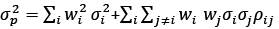(3)

The standard deviation of the portfolio, being a sufficient indicator of risk according to MPT, is influenced by the weights of the assets, correlation and risk of the individual assets. However, T. Morien (2005) disagrees, saying that standard deviation does not reflect all types of risk. Standard deviation of a portfolio represents a square root of variance:

(4)

2.1. Mean Variance portfolio

The efficient frontier can be estimated applying quadratic programming problems:

max w^Tμ (5)

or

min w^T ∑ μ

subject to constraint: 𝑤 ^𝑇𝑤 =1,

where w^T represents a vector of weights, allocated to each asset in the portfolio, ∑ is the variance-covariance matrix of the asset return. By solving those problems, we can estimate the lowest possible risk within the maximum reward (Markowitz, 1952, 1959).

2.2. Risk Parity portfolio

The idea of risk parity was introduced by Bridgewater Associates in 1990s. Originally, a portfolio was considered to be in parity when the weights were equal to the asset class inverse volatility. For instance, if “subportfolio” of equity has a volatility of 9% and a fixed income “subportfolio” has a volatility three times lower, of 3%, then the merged portfolio has to be allocated as 75% of fixed income and 25% of equity to form a parity. This initial concept of a parity portfolio omits correlations, even if there are more than two assets in the portfolio (Clarke, Silva & Thorley, 2006).

According to J. Kanapeckas – the Head of the Risk Management and Reporting Division of the Bank of Lithuania – Lithuanian Bank was among the first central banks to apply the modern risk parity method. The approach guarantees equivalent allocation of risk, enlarges stability during financial downturns and leads to higher expected gains within medium or longer duration periods (Lietuvos bankas, 2017).

2.3. Statistical Moments

There are four statistical moments. Mean, being a location operator of the distribution is presented as:

(6)

The second moment is variance :

(7)

Because of the fact that variance measures the square of the fluctuations from the mean, it is not sensitive to the direction. The third statistical moment is skewness. Skewness estimates the standardized deviation, raised to the third power. It is defined as:

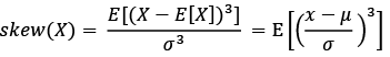(8)

The fourth statistical moment is kurtosis. Kurtosis, being a unit -free statistical measure, can be defined similarly as skewness, except that for the estimation of kurtosis the fourth power of standardized deviation is raised. The positive power indicates that kurtosis is sensitive to positive as well as negative fluctuations of a financial instrument. A random variable, which is normally distributed, has skewness of zero and kurtosis equal to three (Hudson & Mandelbrot, 2010). Kurtosis is defined as:

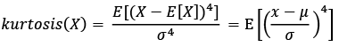(9)

Since the 2008–2009 downturn, traditional financial theories have been criticized for incapability to realistically explain risk. Classical methods of asset pricing usually are built upon a normal distribution, however, in reality the market hardly does follow the bell curve. L. Klebanov and I. Volchenkova (2015) analyzing time series admitted that a majority of indexes, such as Dow Jones Industrial Average index and daily ISE-100 Index within the period of their research transcend the 99% confidence interval on the mean and even more overstep ±5% from the average and fall outside ±10% of standard deviation. Though, it can be summed up that observations do not agree with the assumption of normality and are rather fat-tailed. Since 1963, when B. Mandelbrot encountered fat-tailed distributions among certain financial sequences, it was suggested to consider heavy-tailed models of return of financial assets. The growing popularity of derivatives is a result of nonnormality of the distribution of financial returns became a usual process of risk hedging, rather than a statistical problem (Cherubini, Luciano & Walte, 2004).

Under the assumption of normal distribution, a bell-shaped curve, which is characterized by zero mean and constant variance, the density function of a normally distributed variable x with a mean μ (location parameter) and standard deviation σ (scale parameter):

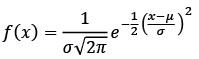(10)

Values that are located close to the center of the distribution have a higher opportunity to occur, while values located close to the tails have less chances to occur (Weisstein, 2002). Presence of fat tails in the distribution is called leptokurtosis. Existence of outliers means the risk of downturn. Because of the fact that the magnitude of the events is hardly predictable, left tail events can have crushing consequences on the return of portfolios (Anson, 2008). In fat-tailed distribution extraordinary events can have a disproportionally high influence on determining assets. For the normal distribution N. N. Taleb (2018) admits that a sequence of very extreme events needs to happen not a single one. “Black Swans” are rather successive than frequent. The fattest tail has a single very large outlier, rather than many deviations from the normal distribution. N. Taleb suggests accidently selecting two people with a merged wealth of $36 million. He admits that the most possible combination is not $18 million and $18 million, though it is roughly $35,999,000 and $1,000, which indicates a large contrast between the two spots. Therefore, a crash can result not from a series of bad events, but from one remarkable accident (Taleb, 2019).

2.4. Value at Risk

Back in 1990, the new CEO of JP Morgan D. Weatherstone requested to deliver him an updated report of risk of the company every day, in a particular time. Known as “4.15 pm report”, resulted in the establishment of the famous risk measure − Value at Risk (VaR). The report was based on sensitivity calculations developed to take into consideration the offset, correlation and delivery of a concluding number, which would represent the maximum financial loss that could occur over a particular time horizon with a set confidence interval. It is important to highlight that in case the confidence level is reduced, the Value at Risk number would decline as well. Value at Risk needs two parameters: confidence interval and a time frame. The main advantage of Value at Risk is the ability of comparing different lines of businesses. Institutions may hedge this type of risk by keeping the economic capital large enough to deal with possible loss (Morgan, 1996).

The expected shortfall, which is known as CVaR or tail risk, measures the weighted average of tail losses that are left beyond the VaR. CVaR is a coherent risk measure. P. Artzner, F. Delbaen, J. Eber and D. Heath examined the coherency of measures more deeply. According to them, the coherent risk measure has to be distinguished by the following four properties. Firstly, coherence assumes Monotonicity. A portfolio delivers the poorest result compared to another portfolio. Secondly, the translation invariance is common to a coherent risk measure. If a particular sum of funds G is added to a portfolio, its risk measure should reduce by the same amount G. The third property of coherence is Homogeneity. In case of changing the size of a basket by multiplying the amounts of all assets by λ, the risk measure is being multiplied as well by the same amount λ. The final quality of coherence is Subaddivity. While the merging of two random portfolios P₁ and P₂, the risk measure does not exceed the sum of risks of two portfolios P₁ and P₂ (1999). According to Artzner et al. (2013), Conditional Value at Risk has all four qualities. However, VaR may sometimes skip the last property, which assumes a positive effect of diversification. In order to obtain CVaR the weighted average of tail losses taking into account that the VaR threshold has been exceeded:

(11)

3. Methodology

With the aid of the programming software Phyton historical daily closing stock prices data of fifteen financial instruments have been gathered from yahoofinance.com within one-year time horizon from 2019 June 1 till 2020 June 1 for further asset allocation. Among the selected financial instruments, two are commodities: Bloomberg Commodities index and SPDR Gold Shares (GLD) ETF. For safe investments, iShares International Treasury Bond ETF (IGOV) has been chosen, which consists of an index of developed government bonds outside the United States. The second bond market asset that has been selected is Vanguard Total International Bond ETF, which includes major bond markets outside the United States. The third financial asset that exposes fixed payment markets, is iShares iBoxx $ Investment Grade Corporate Bond ETF (LQD). It tracks US-dollar denominated USA corporate bonds. Furthermore, two indexes that track USA corporate equity performance have been chosen. The first index is S&P MidCap 400 (^MDI), which follows Mid Capitalization companies. The second index is Russell 2000 (RUT). The index tracks the smallest companies in Russel 3000. Data of Large Capitalization American companies has been collected. The first company is Nvidia Corporation (NVDA), which operates in Technology sector within the industry of semiconductors. The second company is Amazon Inc (AMZN), whose exposure is in the sector of Consumer Cyclical within an industry of internal retail. Large capitalization companies outside USA have been chosen for the construction of portfolios. Firstly, the Swiss company Givaudan SA (GVDNY), which operates in the sector of Chemicals and focuses on Specialty Chemicals industry. Furthermore, historical stock data of large companies of developing countries, which diversify portfolios as risky assets, have been gathered: Russian Industrial Metals and Mining company – Norilsk Nickel (NILSY), and Tencent Holdings Limited (TCEHY) – a Chinese multinational technology conglomerate, which operates in the sector of Communication services within the industry of Internet Content & Information. Finally, the mutual exchange fund SPDR EURO STOXX 50 ETF (FEZ), which tracks blue-chip European companies’ performance, has been included in the portfolio.

For the research all collected data are hedged in American Dollar currency (USD). For Sharpe ratio estimation a risk-free rate has been considered as zero. Furthermore, return of financial assets have been estimated, where R_t is return of an asset, S_t is a stock price at current period and S_t–1 is the price of the stocks in step back period. All in all, 251 observations have been collected for further construction of portfolios:

(12)

3.1. Risk Parity Portfolio

The target of RP portfolio is the allocation of weights, taking into consideration the marginal contribution of each asset in order to achieve the same contribution to the whole portfolio risk. By building RP portfolio the target has been set to allocate weights for equalizing the risk contribution of each asset within the portfolio: σ_i(w) = σ_j(w) = σ_k(w)… = σ_n(w), where σ_i(w). The solution of the Risk Parity portfolio is a quadratic optimization problem:

(13)

where,

Constraints are the weight restriction w^Tw = 1and prohibition of short selling, 0 ≤ w ≤1. With a programming language RStudio the following results have been obtained. All assets have equal contribution to the whole portfolio, which is equal to 6.667% (see Table 1). σ_i is a mean standard deviation of an asset i, w_i is a weight in percentage allocated by optimization process to a financial instrument i.

(14)

where ∂σ / ∂w_i = (∑w)_i is a marginal contribution of an investment instrument. Weighted marginal contribution w_i × ∂σ / ∂w_i represents the component contribution of an asset. In accordance with the Euler’s theorem, the sum of component contributions is equal to the total portfolio risk:

(15)

Standard deviation of the portfolio based on daily collected data can be estimated by taking a square root of transposed vector of weights multiplied by the covariance matrix and multiplied by a vector of weights: σ_{w daily} = 0.279%, which is equal to the sum of component contributions of the assets. The return of the portfolio can be estimated by calculating a product of a vector of weights and a vector of expected return: R_p = 0.026%. Annualized standard deviation and Sharpe ratio, respectively, have been obtained by multiplying the daily results by a square root of the number of periods – the number of trading days within one-year horizon. Using RP portfolio technique, the following results have been obtained (see Appendix 1).

Table 1. Risk Parity portfolio analysis

No.	Ticker	σi	wi	φi(w)	∂σ / ∂wi	wi × ∂σ / ∂wi
1	AMD	3.59%	0.78%	6.667%	2.497%	0.01967%
2	AMZN	1.97%	1.63%	6.667%	1.214%	0.01979%
3	^BCOM	1.05%	3.36%	6.667%	0.59%	0.01982%
4	BNDX	0.31%	10.78%	6.667%	0.184%	0.01984%
5	DX-Y.NYB	0.42%	39.95%	6.667%	0.05%	0.01998%
6	FEZ	2.12%	1.17%	6.667%	1.686%	0.01973%
7	GLD	1.11%	4.23%	6.667%	0.468%	0.00198%
8	GVDNY	0.52%	27.36%	6.667%	0.072%	0.01970%
9	IGOV	1.08%	3.72%	6.667%	0.532%	0.01979%
10	LQD	2.45%	1.07%	6.667%	1.848%	0.01977%
11	^MID	3.26%	0.83%	6.667%	2.374%	0.01970%
12	NILSY	3.54%	0.79%	6.667%	2.548 %	0.01987%
13	NVDA	2.54%	1.02%	6.667%	1.943%	0.01982%
14	^RUT	2.20%	1.33%	6.667%	1.492%	0.01984%
15	TCEHY	0.52%	27.36%	6.667%	0.072%	0.01970%
	∑w		100%	100%		0.279%

Reference: Author’s.

3.2. Global Mean Variance Portfolio

In this paper the global minimum variance portfolio has been constructed, which targets to reduce the total risk. The following optimization task has been set:

min 𝑤 ^𝑇 ∑𝑤 (16)

subject to constraints:

0 ≤ w ≤ 1

𝑤 ^𝑇 𝑤 = 1,

where 𝑤^T represents a vector of weights, allocated to each asset in the portfolio, ∑ is the variance-covariance matrix of asset’s return. With the assistance of optimizer and programming language Python the vector of weights has been obtained. As a result of optimization, the main emphasis has been put on the cash market, allocating 55% into US dollar index, 42% into iShares International Treasury Bond ETF and 3% into Bloomberg Commodities Index.

3.3. Maximum Sharpe Ratio Portfolio

By setting the target of Tangency portfolio, it has been aimed to maximize the equilibrium between risk and reward.

(17)

Restrictions are prohibition of short selling 0≤ w ≤1 and, in order to create full portfolio, the sum of weights has to be equal to one w^Tw = 1. In this portfolio we do not apply any restrictions on minimum of required return. The optimized basket (see Appendix 1) includes six financial instruments, investing 40% in gold, more than the fourth part of the investment has been allocated to US Dollar Index, while Nvidia Corporation has received almost 15%, and 11% has been put into Vanguard Total International Bond Index Fund ETF. Very small amount has been allocated to iShares International Treasury Bond ETF and Givaudan ADR. The Tangency portfolio consists of 18% equities, 16% fixed payment assets, 25% cash, 41% commodities.

3.4. Portfolio Optimization applying Monte Carlo Simulation

Employing the programming language Python, code suggested by S. Jamieson (2019), the Monte Carlo simulation (MS ) has been run assigning random weights, the sum of which is equal to one. In order to achieve more accurate results, 20 000 random portfolios have been generated. From the great majority of the created portfolios, the most optimal have been chosen in accordance with the goals: Maximum Sharpe ratio portfolio (MS), Global Mean Variance portfolio (MS), Maximum Return portfolio (MS). The constraints assume only buying stocks, hence, the minimum weight allocated to an asset i has to be equal or be more than zero. Moreover, the sum of weights has to be equal to one. In accordance with the MS technique, all assets receive at least a small fraction of weight.

Comparing the Sharpe ratio (SR) of the above discussed portfolios. The annualized SR of the Tangency portfolio is equal to 2.01, which is considered to be a good option. The GMV portfolio has a very low annual Sharpe ratio, reaching only 1.22. Comparing the annual SR with the same performance measure of the Risk Parity portfolio, it has been noticed that the Tangency portfolio’s annual Sharpe ratio is 45% higher than the SR of the Risk Parity portfolio. The Maximum Return portfolio exceeds by 21% the Sharpe ratio of the Risk Parity portfolio. While the Minimum Variance portfolio is 11% lower than the SR of the Risk Parity portfolio.

Fig. 1 displays the optimal portfolios in accordance with previously set targets. x axis indicates the annual deviation from the mean of portfolios, while y axis determines the expected annualized return of the portfolios. The great majority of dots indicates dynamically simulated portfolios, the sum of which is twenty thousand. The scale, located on the right side of Figure 1 illustrates the annual return from the lowest to highest. As a result of dynamic simulation, the optimal portfolios have been selected. The green star sign indicates the GMV portfolio; red star shows the Tangency portfolio; yellow sign stands for the Maximum Return portfolio.

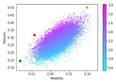
Fig. 1. Portfolio optimization applying the Monte Carlo simulation

Reference: Author’s.

3.5. Minimum Value at Risk Portfolio

Using a dynamic optimization technique with the aid of the programming language Python, the code suggested by S. Jamieson (2019), an optimal portfolio targeting to reduce VaR has been constructed by minimizing the parametric Value at Risk under 99% confidence interval.

VaR = R_p − (z × σ_w), (18)

where R_p is a portfolio expected return, σ_w is a risk of the portfolio and z is a critical value, or value of the cumulative distribution function of Gaussian distribution. The achieved results reveal that annualized return of the portfolio is high, reaching 32.44%, standard deviation is 17.57%. The Minimum VaR portfolio has produced the annual Sharpe ratio of 1.84. Optimization of Value at Risk has several disadvantages: it is not convex, not coherent, not linear.

The star sign indicates the Minimum Value at Risk portfolio (see Fig. 2), which has been chosen as optimal between a great majority of stochastically simulated portfolios. x axis indicates the VaR of one year with a confidence level of 99%, y axis measures the expected annualized return of the portfolio.

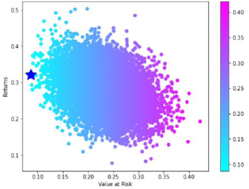
Fig. 2. Portfolio optimization. Min VaR portfolio, based on the MC simulation.

Reference: Author’s.

3.6. Mean Absolute Deviation Portfolio

Mean-Absolute Deviation (MAD) is an alternative to Mean-Variance model. MAD portfolio has a set of advantages over MV portfolio. Firstly, it does not assume the normal distribution of stock returns. Secondly, for the construction of MAD the covariance matrix is not needed. The objective of MAD is minimization of deviation, which can be expressed as LP problem, where n is the number of observations, r_i is a daily return of the asset i, μ_i is a mean daily return of the i asset, w_i stands for the percentage of weight of this asset. The optimization objective has been set:

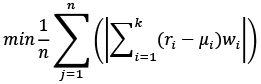(19)

subjects to constraint are:

μ^T w ≥ R

w^T w = 1

w ≥ 0

Analyzing the basket of MAD, it has been noticed that the optimization process has resulted in the allocation of more than 67% of the investment in gold, while Nvdia corporation has received almost 7% of weight, Swiss company Givaudan SA has received almost 8% of weights. All other twelve assets have received almost equal amount of weights, estimating from 1% to 2% each. During the optimization process, all assets have been included in MAD portfolio.

3.7. Minimum CVaR Portfolio

In this paper the linear programming approach suggested by A. Charnes and W.W. Cooper (1962) has been applied. Using the programming software Python, the solution to the following mathematical problem has been found in order to minimize the expected shortfall:

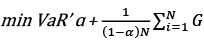(20)

subjects to constraint:

G ≥ 0

w^T w = 1

w ≥ 0,

where VaR is a historical value at risk, ɑ is an upper quantile of a loss function, which is equal to 1%; w_i stands for the percentage of weight of this asset; G is an auxiliary variable, representing the values exceeding the VaR. The Minimum CVaR portfolio has produced even higher return than the Maximum Sharpe Ratio portfolio, reaching 31.96% annually. It is the third highest return after the Maximum Return portfolio, based on the Monte Carlo simulation and the previously discussed MAD portfolio. Analyzing the standard deviation, it has to be highlighted that the total risk of CVaR portfolio is lower than the volatility of VaR portfolio. The standard deviation of CVaR portfolio being 15.78% annual is almost in line with the standard deviation of the Tangency portfolio based on the Monte Carlo simulation approach. The same refers to the Sharpe ratio, which is almost equal to the SR of the Tangency portfolio based on the Monte Carlos approximation. The basket of CVaR portfolio consists of more than 80% in gold, a remarkable percentage of weight − 5.09% – has been allocated to Nvdia corporation, while all other weights have been spread almost equally to all thirteen financial instruments.

4. Performance evaluation of the Portfolios

4.1. Sortino Ratio

In contrast to Sharpe ratio, Sortino ratio penalizes the return that is less than the minimum required return. Sortino ratio is defined as

(21)

where R_p stands for a portfolio return; MAR is minimum accepted return; σ_d is downside deviation. For the calculation of Sortino ratio, the following steps have been fulfilled. The monthly data of market return of S&P500 have been collected and a mean monthly return of 0.76%, as a benchmark of minimum accepted return, has been obtained. The monthly return of each previously created portfolio has been calculated by the sum of the weighted average of the monthly expected returns of each asset in accordance with the previously allocated weights. Secondly, periods with negative returns have been selected for each portfolio, while periods with positive returns have been omitted. Thirdly, the negative returns of each period for each portfolio have been squared and summed. The highest downside risk is typical to the Equal Weight portfolio, it reaches 0.0293. The lowest downside risk has been observed to have Maximum Sharpe Ratio portfolio based on the quadratic optimization technique. It is interesting to mention that the downside risk of Maximum Sharpe Ratio portfolio based on the Monte Carlo optimization approach is more than two times bigger than the downside risk of the same target portfolio constructed using the quadratic programming technique – 0.016 and 0.07 respectively. It is important to highlight that Minimum VaR portfolio has a higher downfall risk than Minimum CVaR portfolio. It has been obtained that the Maximum Sharpe Ratio portfolio, based on the quadratic portfolio technique, has a remarkably higher Sortino ratio in comparison with the values of Sortino ratio for other created portfolios. The second highest position belongs to the MAD portfolio, estimated as 8.939. It is interesting to highlight, comparing Maximum Sharpe ratio portfolios, that the one which is based on the Monte Carlo simulation optimization technique, has more than two times lower Sortino ratio than the same portfolio based on the quadratic optimization technique. Analyzing the portfolios that target to hedge risk, such as Minimum VaR and Minimum CVaR portfolios, it has been noticed that the former portfolio has a higher Sortino ratio than the Minimum Value at Risk portfolio.

Table 2. Annualized Sortino ratio of created portfolios.

Portfolio/ Ratio	EW	RPP	Max SR	GMV	Max SR (MS)	MV (MS)	MR (MS)	Min VaR	MAD	Min CVaR
Downside Risk	0.029	0.011	0.007	0.009	0.016	0.022	0.023	0.017	0.014	0.014
Sortino Ratio	2.79	1.76	12.39	0.24	5.88	1.90	6.43	5.54	8.91	5.88

Reference: Author’s.

4.2. Treynor Ratio

In order to compare the performance of all portfolios in terms of the Treynor ratio, the following steps have been performed. Firstly, the beta of each asset has been calculated as the covariance of asset i with market and divided by variance of the market:

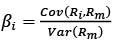(22)

For obtaining the beta of the portfolio (β_p) transposed vector of weights (w₁… w₁₅) of each asset has been multiplied by the matrix of individual betas(β₁… β₁₅) of each asset. Then, in accordance with the formula, the Treynor ratio has been calculated:

(23)

where R_p is return of the portfolio and β_p is beta of the portfolio.

Table 3. Portfolio beta and Treynor ratio.

Portfolio / Ratio	EW	RPP	Max SR	GMV	Max SR (MS)	GMV (MS)	MR MS)	Min VaR	MAD	Min CVaR
Treynor Ratio	0.46	0.57	1.22	1.33	0.77	0.47	0.61	0.67	1.10	1.72

Reference: Author’s.

Analyzing the obtained results of Treynor ratio (see Table 3), it has been noticed that the Minimum CVaR portfolio has the highest value of Treynor ratio, which can be interpreted as this portfolio has the best risk-adjusted return in comparison to return of the other constructed portfolios. The lowest capacity against market belongs to the Equal Weight portfolio, having more than three times lower result in comparison with Treynor ratio of Minimum CVaR portfolio.

4.3. Location and Variability of the Portfolios

In order to characterize the location and the variability of return of each portfolio (see Table 4), third and fourth moments − skewness and kurtosis – have been estimated. Skewness, being a third power of deviation is especially sensitive to negative fluctuations. The highest value of skewness is typical to the Risk Parity portfolio, which signalizes that this type of portfolio has produced more negative fluctuations. Moreover , the negative skewness of two indicates that the data are negatively skewed and the left tail of the distribution is longer, while most of the data are located on the right side. Equal Weight, Maximum Sharpe Ratio (MS), global Mean Variance (MS) and Min VaR portfolios’ returns are highly skewed, hence, most of the data being asymmetrical are located on the right-hand side of the distribution and has a longer left tail. While Maximum Return portfolio (MS), having skewness of –0.77, produces moderately skewed return. Having skewness less than |0.5|, the distributions of return of the global Mean Variance, Max Sharpe Ratio, MAD, Min CVaR portfolios are fairly symmetrical. It is important to highlight that the Maximum Sharpe Ratio portfolio based on the Monte Carlo approximation technique has highly skewed returns, while the same portfolio based on the quadratic optimization has almost symmetrically skewed returns.

Table 4. Moments of the composed portfolios.

Portfolio	EW	RPP	GMV	Max SR	Max SR (MS)	GMV (MS)	MR (MS)	Min VaR	MAD	Min CVaR
Skewness	-1.1	-2.0	-0.5	-0.03	-1.15	-1.72	-0.77	-1.09	-0.04	0.19
Kurtosis	10.3	13.7	2.78	10.15	11.16	11.73	7.87	10.86	11.84	6.98

Reference: Author’s.

The statistical analysis has revealed that only Minimum CVaR portfolio has positive skewness. The former fact leads to the interpretation that the Minimum CVaR portfolio has mode which is smaller than the mean and median. While all other created portfolios have the negative skewness of their return’s distribution, which indicates that the mean and median will be lower than mode.

Being a fourth power of deviation, kurtosis reveals positive, as well as negative fluctuations. It can be noticed that Global Mean Variance portfolio has kurtosis of less than three, therefore, the distribution of its returns has fewer outliers than a normal distribution does have. Consequently, this portfolio may be desirable for investors in terms of risk hedging, because there is less chances of encountering severe losses. Remarkably, the highest kurtosis, as well as the previously described large skewness, are typical to the Risk Parity portfolio return. It reaches more than 13, which indicates that the distribution of its return has fat tails and may have much more than usual extreme events.

4.4. Value at Risk of the Portfolios

Downside risk measure has been applied to the created portfolios. Profit/loss of a portfolio, corresponding to each trading day during estimated period has been calculated. All in all, 251 observations represented by profit/loss have been obtained for each constructed portfolio:

VaR (α) = R_p(t) × I, (24)

where R_p(t) = w^T μ is return of the portfolio in period t, I stands for assumed investment. Secondly, for the calculation of VaR 95%, the worst 5% result of return has been selected between the worst losses of each portfolio during the analyzed time horizon. The following results of VaR with α = 5% have been observed (see Table 5).

Table 5. One day historical VaR 95%. All values are presented in percentage (%).

Portfolio	EW	RPP	Max SR	GMV	Max SR (MS)	GMV (MS)	MR (MS)	Min VaR	MAD	Min CVaR
VaR 95%	1.8	0.34	0.92	0.20	1.17	0.916	2.70	1.33	1.37	1.35

Reference: Author’s.

Taking into consideration the results of historical VaR 95%, it has been noticed that the lowest losses are typical to the GMV portfolio. It can be interpreted that with a confidence level of 95%, the daily loss should not exceed 0.19% of the initial investment. The Risk Parity portfolio has yelled low loss, which has reached only 0.34% of the initial investment. Three times higher Value at Risk 95% has been noticed to be typical to the Global Mean Variance portfolio, based on the Monte Carlo simulation approach. One day Value at Risk of 95% of the Maximum Sharpe Ratio portfolio, based on the quadratic programming technique is almost in line with the former portfolio, which is 0.92%.

4.5. Expected Shortfall of the Portfolios

For the estimation of exceedance, the following steps have been implemented. In Excel program, after the estimation of historic Value at Risk with a confidence level 95%, the matrix C 251×10 has been created, where 251 stands for the number of returns during the estimated time horizon, while 10 indicates the number of portfolios. Secondly, the return of the portfolio, where a value is lower than Value at Risk with a confidence level of 95% has been marked as zero, while the value, which has exceeded the 95% VaR has been marked as 1. Finally, the average value of portfolios exceeding Value at Risk within a 95% confidence interval has been estimated.

Table 6. One day Expected Shortfall, α = 5%. All values are presented in percentage (%).

Portfolio	EW	RPP	Max SR	GMV	Max SR (MS)	GMV (MS)	MR (MS)	Min VaR	MAD	Min CVaR
CVaR 95%	3.63	0.74	1.64	0.32	2.49	2.02	4.78	2.80	2.50	2.16

Reference: Author’s.

It is important to emphasize that the portfolio, which targets to minimize Value at Risk, has worse results than the Minimum CVaR portfolio. The Minimum Value at Risk has higher tail loss than the Mean Deviation portfolio. The highest downfall is typical to the Equal Weight portfolio and the maximum return portfolio, estimating 3.68% and 4.78% daily tail loss accordingly. It is interesting to mention that all portfolios based on dynamic optimization have rather higher tail loss than the same portfolios based on quadratic optimization technique.

4. Conclusions

In light of the previously discussed conducted academic research, main observations have to be emphasized. It has been observed that the distribution of returns of the Risk Parity portfolio has the biggest negative skewness. It leads to the conclusion that the Risk Parity portfolio has performed a lot of small gains and a couple of extreme outcomes have been encountered. Almost the same performance has been typical to the GMV portfolio based on the Monte Carlo simulation and the Equal Weight portfolio. It is interesting to note that in terms of location, the Highest Return portfolio, which has three times lower negative skewness, in comparison with the Risk Parity portfolio’s skewness, which means it has less extremes. Secondly, it has to be stressed that only the Minimum CVaR portfolio does have a positive skewness, which means that in comparison with other portfolios, it has more small losses and few large profits. It is important to accent that all portfolios, constructed applying the Monte Carlo simulation technique, have higher negative skewness than the portfolios with the same targets, based on the quadratic optimization technique.

After the academic analysis of the created portfolios, one of the highest kurtosis and, hence, heavy tails have been encountered to have the Minimum Value at Risk portfolio. Taking into consideration the results of location and the variability of the return of the constructed portfolios, the Risk Parity portfolio, has the highest kurtosis and the biggest skewness, hence, this technique may reduce the standard deviation, however, few extreme outliers may occur.

Analyzing the third performance ratio – Sortino ratio, it has been noticed that the best result has been obtained by the Maximum Sharpe ratio portfolio based on the quadratic optimization technique. Comparatively high results have been achieved by the Minimum CVaR portfolio. While, the Maximum Sharpe ratio portfolio, based on dynamic optimization, has produced even lower results than the Minimum VaR portfolio.

Taking into consideration the Treynor Ratio, evaluating the performance of the created portfolios, it has been found out that the lowest capacity against the overall market has been typical to the Equal Weight portfolio. While the minimum CVaR portfolio has produced the highest results, which indicates that the strongest capacity against the overall market belongs to the Minimum CVaR portfolio.

The best capacity against downside deviation has been achieved by the Maximum Sharpe ratio portfolio, based on the quadratic optimization technique. The worst resistance against downside deviation has been obtained by the Global Mean Variance portfolio.

Taking everything into consideration, the Minimum CVaR portfolio may be a perfect option for investors who want to increase the return and hedge two types of risk: standard deviation and rare severe negative losses. This type of portfolio has lower kurtosis and almost symmetrical distribution and comparably good return and low dispersion. CVaR is a more accurate technique for risk hedging than Value at Risk.

References

Anson, J.P. (2008). Handbook of Alternative Assets. United States: John Wiley & Sons, 720 p.

Artzner, P., Delbaen, F., Eber, J. & D. Heath. (1999). Coherent Measures of Risk. Mathematical Finance, Vol. 9, issue 3, p. 203–228. https://doi.org/10.1111/1467-9965.00068

Charnes, A. & Cooper, W.W. (1962). Programming with linear fractional functionals. Naval Research Logistics Quarterly, Vol. 9, issue 3–4, p. 181–186. https://doi.org/10.1002/nav.3800090303

Cherubini, U., Luciano, E. & Vecciato, W. (2004). Copula Methods in Finance. United States: John Wiley & Sons, 310 p.

Clarke, R. G., De Silva, H., Thorley, S. (2006). Minimum Variance Portfolios in the U.S. Equity Market. Journal of Portfolio Management, Vol. 33, issue 1, p. 10–24. http://dx.doi.org/10.3905/jpm.2006.661366

Herbener, J. M. (2011). The pure time–preference theory of interest. United States: Ludwig von Mises Institute, 189 p.

Jamieson, S. (2019). Minimization of Value at Risk. Retrieved from https://pythonforfinance.net/

Lietuvos bankas. (2017). Bank of Lithuania is improving investment policy to effectively manage investment risk and earn higher return in the longer term. Retrieved from https://www.lb.lt/en/news/bank–of–lithuania–is–improving–investment–policy–to–effectively–manage–investment–risk–and–earn–higher–return–in–the–longer–term

Markowitz, H. (1952). Portfolio Selection. The Journal of Finance, Vol. 7, issue 1, p. 77–91. https://doi.org/10.1111/j.1540-6261.1952.tb01525.x

Markowitz, H. (1959). Portfolio Selection: Efficient Diversification of Investments. New York: Wiley.

Mintz, M. (2020). COVID–19 Daily Update. S&P Global. Retrieved from https://www.spglobal.com/en/research–insights/articles/daily–update–november–30–2020

Morgan, J.P. (1996). RiskMetrics Technical Document. (4th ed.). J.P. Morgan, New York.

Morien, T. (2005). Travis Morien Financial Advisors. MPT criticism. Retrieved from https://www.lapasserelle.com/escem/finance1/13_portfolios_(2)/Modern%20Portfolio%20Theory%20criticisms.htm

Hudson R. L, B. Mandelbrot (2010). The (Mis)Behaviour of Markets: A Fractal View of Risk, Ruin and Reward. England: Profile Books.

Reilly, F. K & Brown K.C. (1999). Investment Analysis and Portfolio Management. 6th Edition, United States: South-Western Cengage Learning.

Special Focus. (2020). A Shock Like No Other: the Impact of COVID–19 on Commodity Markets. Publishing and Knowledge Division, World Bank internet access: http://pubdocs.worldbank.org/en/558261587395154178/CMO–April–2020–Special–Focus–1.pdf

Spitzer, S., Wiedemer R.A., Wiedemer., D. (2009). Aftershock: Protect Yourself and Profit in the Next Global Financial Meltdown. 4th edition. United States: Wiley Hoboken.

Taleb, N. N. (2018). Skin in the Game. United States: Random House, 272 p.

Taleb, N. N. (2020). Statistical Consequences of Fat Tails. Stem Academic Press, 446 p.

Weisstein, E.W. (2002). Normal Distribution. From MathWorld. Retrieved from https://mathworld.wolfram.com/NormalDistribution.html

Appendices

Appendix 1. Constructed portfolios and evaluation of their performance.

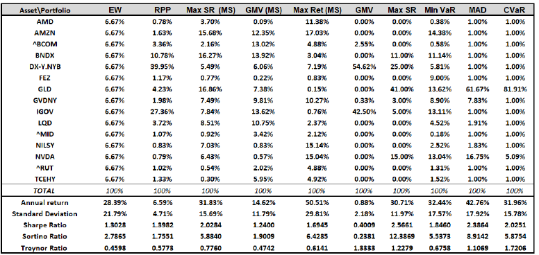
Reference: Author’s.

Appendix 2. Distribution of returns of the Portfolios and VaR 95%, CVaR 95%.

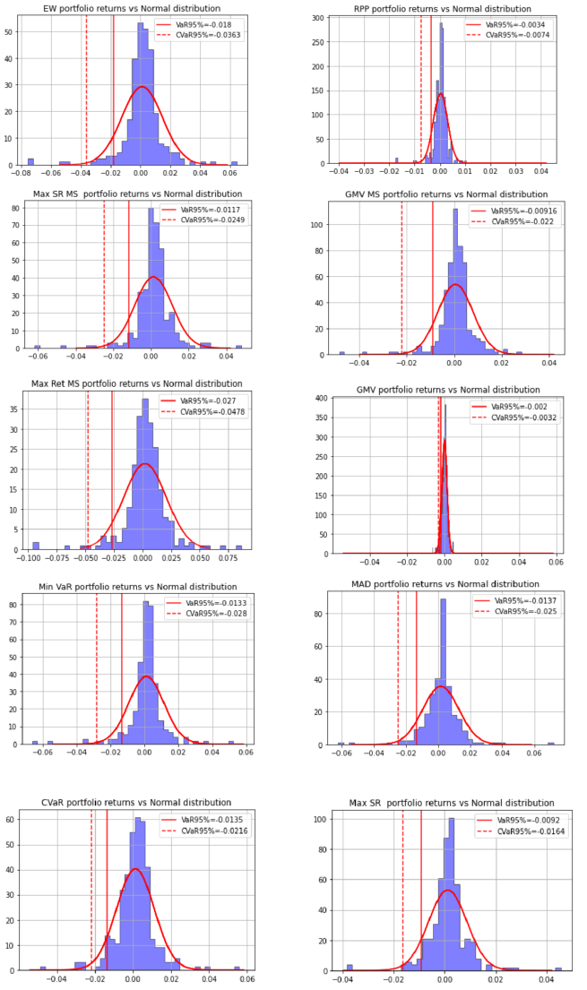
Reference: Author’s.