Ekonomika ISSN 1392-1258 eISSN 2424-6166
2021, vol. 100(2), pp. 84–100 DOI: https://doi.org/10.15388/Ekon.2021.100.2.4
Estimates of Russia’s Potential Output
Petr Maleček
Faculty of Economics, Prague University of Economics and Business, Czech Republic
E-mail: petrxmalecek@gmail.com
Martin Janíčko
Faculty of Economics, Prague University of Economics and Business, Czech Republic
E-mail: martin.janicko@email.cz
Pavel Janíčko
College of Regional Development and the Banking Institute – AMBIS, Czech Republic
E-mail: janicko.pavel@cmkos.cz
Abstract. Considering the specifics of the Russian economy such as dependency on oil, gas drilling and production, including the current context of the Western sanctions, COVID-19 pandemic as well as distinct potential output development, the main aim of this paper is to quantify the recent output gap for Russia. We use three mainstream methodologies: the Hodrick-Prescott filter as a benchmark, the Kalman filter to follow and the Cobb-Douglas production function. The sample time span ranges from 1995Q1 until 2020Q3, while all calculations are performed on quarterly frequencies. The analysis suggests that given the low fixed investment ratios, limited R&D spending in non-military sectors and adverse demographic development, under a “no policy change” scenario, there might soon be even more downward pressures on the country’s potential output growth. The economy may continue increasing only at a snail’s pace even after a possible withdrawal of the Western sanctions and the end of the COVID-19 pandemic.
Keywords: Russian economy; potential output; production function; Hodrick-Prescott filtering; Kalman filtering
_________
Received: 16/02/2021. Revised: 24/04/2021. Accepted: 26/04/2021
Copyright © 2021 Petr Maleček, Martin Janíčko, Pavel Janíčko. Published by Vilnius University Press
This is an Open Access article distributed under the terms of the Creative Commons Attribution License, which permits unrestricted use, distribution, and reproduction in any medium, provided the original author and source are credited.
1. Introduction
Russia’s economy has not been faring well as of late. In particular, the Western sanctions following the annexation of Crimea and relatively weak energy prices have been the main culprits of the general economic slowdown, manifested itself by the recession in 2015, followed by a lacklustre GDP growth until now.
Looking at a longer time span, the country already had to overcome major financial and economic crisis in 2008 and 2009, while prior to that it had been coping with major economic and social turbulences caused by abrupt privatization by a handful of chosen oligarchs, swift liberalization, frequent intentional dismantlement and/or weakening of elementary institutional mechanisms, and exploding corruption during the 1990s. Also, the skyrocketing inequality in the same period, partly propelled by lifting price controls over 90% of traded goods, made things even worse. These were exactly the problems that resulted in huge output losses and significant social and political unrest between 1992 and 1996, peaking with the 1998 financial crisis, which itself went straight to university textbooks on finance and economics. For illustration, in the time span of 1990 and 1998, Russia’s real GDP plummeted by approximately 45% (World Bank, 2021).Yet, with the beginning of the new millennium, Russia started to be perceived as a relatively normally functioning emerging economy which was achieved inter alia by overall institutional stabilisation and rising openness of the economy to international trade and investment inflows. Still, the rising oil price was likely the chief factor in the country’s economic development between 2000 and 2008, while the high oil price supported the economy also beyond that period, particularly between 2010 and the first half of 2014, after it reached an all-time high in 2013 (Kluge, 2019).
Left aside the difficult access to the global financial markets as well as subdued oil prices, the most pronounced, purely domestic, challenge will perhaps be the negative demographic trend and population ageing (although demographic trends might sometimes be less straightforward than conventionally thought (Blanchard & Quah, 1989)), which is for the time being partially mitigated by immigration flows particularly from the former Soviet republics. Russia’s working-age population declined by around one million during the last years, although employment stagnated in the same period. This heavily weighs on the country’s labour component of the aggregate production function and may even worsen the situation in the years to come unless the labour force is compensated elsewhere: according to the United Nations, the working-age population may drop to only about 90 million in 2030 (UN World Population Aging Report, 2019). Only recently did the government hike the legal retirement age by five years to 60 and 65 for females and males, respectively. The main upside of the shrinking labour force is that the unemployment rate stays low even during recessions as labour becomes relatively scarce with respect to to other production factors. This could be seen during both the Great Recession in 2008 as well as the current situation in which the headline unemployment rate remains below 7% in 2020 (ROSSTAT, 2020), an enviable value for many Western European countries.
The economy remains heavily dependent on oil drilling/production and the share of exports of natural resources of various kinds fluctuates between 16 and 20% (OECD Database, 2021). At the same time, natural resources account for about 80 to 85% of total exports (OECD Database, 2021). Russia’s reserves-to-production ratio stands at 20, while it reaches 89 in Kuwait and 64 in Saudi Arabia (Worldometer, 2021). Meanwhile, the gross capital formation remains low compared not only to the Western countries, but also to the Eastern and Central Europe. This is deemed quite surprising, namely given the general need for higher investment in drilling and extraction. Hence, such lack of productive investment combined with several other negative factors, predominantly present in the institutional functioning of the country, may potentially prevent Russia’s GDP growth from accelerating further and will likely require an appropriate economic policy action.
As for 2020, the Russian economy is estimated to have declined by 3.1% - the most since 2009 (IMF, 2021). The country’s economic development was adversely affected by the coronavirus pandemic and falling oil prices. Russia is expected to return to growth in 2021 and 2022 (IMF, 2021). According to the World Bank (2020), the health crisis caused by the COVID-19 pandemic slowed down the business activity in the country, but also the demand for oil, Russia’s main export commodity. The unemployment rate in Russia rose sharply in response to restrictions on movement imposed throughout the country to prevent the spread of coronavirus. However, even with a positive outlook for further growth, GDP will not reach pre-pandemic levels sooner than in late 2022.
We show that the estimation of Russia’s potential output can be performed with three standard methods, namely Hodrick-Prescott filter, Kalman filter, and the Cobb-Douglas production function with constant returns to scale. All approaches show relatively similar results and identify a negative output gap in Russia’s economy in 1999, 2003, 2009, 2015 and 2020. The results also suggest the economy might begin entering a protracted period of low-potential growth due to low capital-labour ratios, dismal demographics and slow increases in total factor productivity.
We consider the estimation of current growth of Russia’s potential output as the article’s main contribution to the relevant research field. The main contribution particularly resolves the scarcity of up-to-date estimates in this respect which is discussed more broadly in the third section. Furthermore, the value added of this paper lies within disentangling the causes of sluggish growth even before the COVID-19 pandemic, principally by means of decomposition of growth into cyclical and structural factors. With respect to the latter, we also perform a deeper analysis considering developments in the capital accumulation and the labour market. The main novelty of the article resides in the following: we connect the theoretical underpinnings, actual economic situation and quantitative methods to come up with consistent estimation of Russia’s potential output over a relatively long time horizon. Likewise, we analyse three potential output methods, compare and contrast them where necessary. Finally, we use the most up-to-date data allowing us to identify the main episodes and underlying characteristics, stemming from labour market and elsewhere affecting the potential output development. We also believe that, given the relatively consistent results, the methods we used have proved to be appropriate. The text can be useful in offering a reasonable snapshot on Russia’s potential output for the researchers, experts and/or policy makers since, to the best of our knowledge, no other text with similar complexity exists until now.
The rest of the article is structured as follows: the next section explores the major structural issues of Russia’s economy in the current macroeconomic context. Section 3 presents previous research conducted on the topic and the data used. Section 4 details the estimation methods. Section 5 summarises results and provides their comparison. The last section concludes the analysis.
2. Russian Economy: Structural Issues
After seven straight years of expanding at a relatively decent clip, fuelled by increasing oil prices as well as prices of other natural resources and reforms which curbed the power of oligarchs and lobby groups, the Russian economy contracted by nearly 2% in 2015 (ROSSTAT, 2020). This is also due to the combination of the weak oil prices and Western sanctions following the annexation of Crimea as well as Russian countersanctions targeting mainly the Western agricultural and food products. Both sets of sanctions have been in place until mid-2020, but, given the current political and geopolitical context, they will likely be extended beyond that period. Still, even in the years before 2015, Russia’s economy decelerated markedly due to a weak fixed capital accumulation, partially driven by the rising and volatile interest rates on corporate loans. As a result, with low profitability and high interest rates, businesses found it hard to finance major investment projects, and even those companies that could invest in Russia, often preferred to invest abroad rather than domestically.
A relative brisk economic policy response helped Russia avoid even more protracted slump, but the country still ranks poorly in the effectiveness of its state administration, judicial independence, property rights and effectiveness of its financial markets. Combined with all the “exogenous factors”, all these shortcomings are weighing on the near-term economic development of the country and it is worth noting that other countries of the so-called BRICS group are currently ranked higher in most of these gauges.
High interest rates on corporate loans and subdued demand for output also prevent the stimulation and picking up of longer-term capital formation. In addition to this, Russia’s entry into the WTO makes it clear that the domestic industries will have to compete with less expensive imports, and that will require higher productivity, diversification and improved competitiveness. In the short run, agriculture, automobile sector, engineering, pharmaceuticals, and industries producing high-tech equipment will be hurt the most by foreign competition. Nevertheless, over the next several years, Russia’s entry into the WTO should enable the country to more efficiently allocate resources within the economy and will contribute to the increase of the competitiveness of the Russian goods and services. Likewise, slowly but surely, increasing oil prices will support the country’s revenues and increase the margin for manoeuvre in case further fiscal expansion is necessary. Finally, the economy has been accommodating to the Western sanctions and developed some sort of self-sufficiency, albeit at relatively high initial costs, including corruption.
Since the economic crisis of 2015 and 2016, the Russian government has recovered its fiscal and monetary reserves in the context of the rising oil and gas prices. However, the government is trying to maintain an acceptable budget deficit and to implement some fiscal adjustments (cuts in pensions and tax increases, toll growth). For example, (Schwabe, 2019) argues that “(…) Russia has also partially shifted reserves from US dollar-denominated holdings to the euro and even to Chinese currency, but also to holdings of gold reserves, which rose to the equivalent of $110 billion. The National Welfare Fund owned by the government is now worth over $120 billion and is expected to soon reach 7 percent of GDP. This is a formal threshold at which the government could start to use part of the funds.” At the same time, the country significantly reduced its external debt, and only this year the combined external debt of the private and public sectors stopped diminishing and again increased to $480 billion (Schwabe, 2019). As such, Russia is in a favourable situation where all foreign debt of private and public entities is fully covered by foreign reserves. This has made Russia more resilient to the new external shocks, such as a further decline in oil prices or new sanctions. It follows that the Russian economy does not have to worry about high instability even at present, when expectations for future growth are not very optimistic. Still, it remains to be seen whether the production in the oil sector will not start declining from 2021 onwards due to depletion of oil fields and a lack of modern technology.
Demographic challenges also threaten Russia’s economic growth. Given the extremely low birth rate in the 1990s, there is currently a shortage of young workers in the labour market, while many baby boomers are entering retirement age. Migration compensated a part of the workforce, but in the period between 2018 and 2020 the number of migrants dropped as Russia became less attractive for migrant workers (Foltynova, 2020). Many of these problems could be mitigated or offset by a suitable economic policy, but it seems that, because of persistent political rigidity and populism, these opportunities are not being properly exploited. The Western economists recommend Russia could invest in education and health care to increase the productivity and longevity of its shrinking workforce. The domestic and international experts have repeatedly submitted this proposal during Putin’s time in power. However, the Russian government continues prioritizing spending on security services and military.
The concern is also how to distribute the ownership structures in the most important sectors to maximize their contribution to effective growth and competitiveness. Viable programs may include large-scale infrastructure projects, mainly government-funded, in the hope that investments and hence economic growth will strengthen in the coming years.
3. Previous Research and Data
Literature devoted to the Russian potential output is rather scarce, and, given the need for recent data, also relatively obsolete and dating mostly to the period before the Global Financial and Economic Crisis (GFC). One of the examples is (Michalides & Millios, 2009) who attempted to estimate Total Factor Productivity shifts in the Russian economy during the time span from 1994 to 2006. They also calculated the potential output and output gap using the Cobb-Douglas production function and the Hodrick-Prescott filter. Equally, some of the previous papers, e.g. (Oomes & Dynnikova, 2006), elaborate on the importance of utilization rates of primary factor inputs. Similarly, (Hanson, 2009) studies the changing structure of the Russian economy and projects its development until 2020-time horizon. Further, (Izyumov & Vahaly, 2008) came up with a study about levels and trends in capital accumulation in the Commonwealth of Independent States (CIS) since their transition to the market/capitalist economies. Focusing on the 1992-2005 period, they have ascertained that Russia remains the most capitalised CIS country with capital-labour ratio (K/L) of about $40,000 per worker. Finally, (Kuboniwa, 2010) discusses the sources of growth in the Russian economy now and during the financial crisis of 1998-1999. She confirms, inter alia, that the country’s performance in manufacturing and trade sectors still heavily depends on the changes in oil prices. Finally, (Zubarev & Trunin, 2017) estimate Russia’s output gap, following the phase-in of the Western sanctions, and suggest that a slowdown in the potential output growth took place. Most of the previous research confirms that Russia’s potential output has been drifting to a slower growth trajectory.
The data used in this paper have been extracted from the Moody’s Analytics historical data platform DataBuffet (raw data can be found in the Appendix) and the Federal State Statistics Service of the Russian Federation. They covered a period between 1995Q1 until 2020Q3, thus partially taking into account also the impact of the COVID-19 pandemic with the onset in the first quarter of 2020. The end of the time series marks the last full year of available data at our disposal at the time of creation of the article. In certain cases, the times series have been extended with predictions in order to receive more precise data and avoid some methodological issues. Where necessary, data have been transformed into the Seasonally Adjusted Annual Rates (SAAR) to account for changes in data caused by seasonal variations.
4. Methods for Estimating Potential Output in Russia
Bearing in mind the several important particularities of the Russian economy, as outlined in the previous section, let us now turn to the estimation of the potential product and the output gap, using quarterly data. We chose three methods that are commonly used in this respect: the Hodrick-Prescott filter, the Kalman filter and the production function.
4.1. Hodrick-Prescott filter
As our reference method, we use the frequently employed Hodrick-Prescott filter. (Hodrick & Prescott, 1997) The idea of this approach is to disentangle real GDP into its trend part and cyclical part by means of penalization of the trend component growth rate. We set the only free parameter (the penalization parameter lambda) to 1600, which has become mainstream while analysing quarterly data. It holds that the larger the penalization parameter, the smoother it yields the trend. In an extreme case of lambda approaching infinity, the series will exhibit a linear trend.
In a conventional representation, real GDP yt is composed of the trend part gt and cyclical part ct, i.e. it has to hold that:
 (1)
(1)
The trend part is then obtained by minimising the equation below with respect to gt. This can be written as follows:
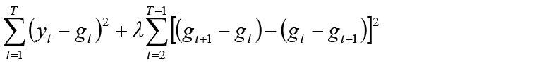 (2)
(2)
4.2. Kalman filter
The Kalman filter or the linear quadratic estimation (LQE), is a significantly more sophisticated method than the Hodrick-Prescott filter. This method is not a purely mechanical filtering technique, but it has more structural character and is recursive. Its use could thus be wide-ranged, and it goes well beyond economics or econometrics. The general set-up of the Kalman filter could be written as follows:
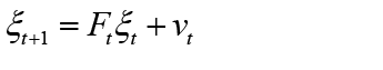 (3)
(3)
 (4)
(4)
where  stands for unobserved variables that are to be estimated, yt represents all observed variables, whilst
  and
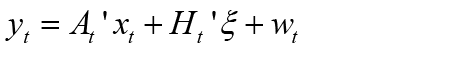
and  are two white noise vectors. Further, Ft , Ht' and At' stand for coefficient matrixes. The main general objective is, based on the initial state x0 with normal distribution and historical observations, to derive optimal estimates of the future states by using maximum likelihood method. In our case, the equation for real output is thus as follows:
 (5)
(5)
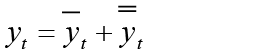
where  is the output gap and
  is the trend. Equation (5) can be further split up into two separate equations – the autoregressive state equation and the trend state equation:
 (6)
(6)
 (7)
(7)
where c1 and c2 are constants and μt is a random variable. On the one hand, the main advantage of the Kalman filter is its ability to consider the effects of all the variables in the model and also the fact that it is less skewed by the historical data than other (statistical) filtering methods. Owing to its structural character, there is also consistency between the model estimates and structural features of the described reality. On the other hand, as it has already been mentioned, the filter is complicated in the sense of initial values for the model. An inappropriate choice of parameters, for example, may partially or completely invalidate the filtering results.
For the Russian economy data, the parameters are calibrated. The state space is defined by the system of equations in the following form:
 (8)
(8)
 (9)
(9)
where νt and et denote independent standard Gaussian variables. In what follows, we consider a standard New Keynesian Model in the following form:
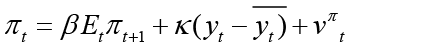 (10)
(10)
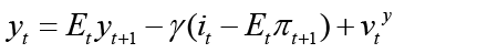 (11)
(11)
 (12)
(12)
 (13)
(13)
where πt denotes the inflation rate, yt stands for the change in the real output, denotes change in the potential output, it is the money market interest rate, and νt and ut stand for normally-distributed estimation errors. The calibrated parameters denoting sensitivities in the system are mostly based on (Kreptsev & Seleznev, 2018) and take the following form:
 (14)
(14)
The solved model is put in the state space form, while changing the variance would affect the behaviour of the Kalman smoothener. For example, smaller variance of measurement errors would put more weight to the variance of structural innovations. According to the filet, the output gap is suggested to be marginally negative as of late, following the events that happened in 2014. Likewise, the filtered series is relatively less smooth than elsewhere which is given by the very nature of the multivariate filter set-up.
As can be observed in Figure 1 further in the text, by using the Kalman filter, the output gap was positive between the years 2000 and 2009, while often hovering around zero or being even negative since that period. In the most recent years, we can see that the gap tends to shrink, which is in line with the recent normalisation of Russia’s GDP growth.
4.3. Production function
To develop upon the statistical nature of the HP filter by gaining more insight into the drivers of potential output growth, the next commonly used method for determining the output gap is the production function. In this paper, we will use the two-factor Cobb-Douglas production function, implicitly treating technological progress as Hicks-neutral, similarly to (d’Auria et al., 2010) and (Giorno, Richardson, Roseveare, & van den Noord, 1995). Thereafter, the potential output is a function of potential capital stock Kt, potential employment Lt, i.e., the level where there should be no demand inflationary pressures, and potential total factor productivity (TFP) At.
 (15)
(15)
In line with the most empirical studies, we will employ constant returns to scale, just as in the original Solow model. According to (Michaelides & Millos, 2009), the labour content of the Russian economy has been stable, oscillating around 50%, we thus set both alfa and beta constant at 0.5. For the capital stock, we use the perpetual inventory method (PIM), which suggests that the current capital stock is the sum of the past capital stock adjusted for depreciation and present real fixed investments. We set the annual depreciation rate to 0.05, in line with several theoretical studies, e.g. (Mourre, 2009). To estimate the potential labour component, we use the convenient decomposition of headcount figures into working age population, trend participation rate and the ‘trend’ unemployment rate that should in theory mirror the non-accelerating inflation rate of unemployment (NAIRU).
 (16)
(16)
The final and vital part is estimating the potential TFP. To keep the method simple enough, we will again consider the potential TFP as a trend TFP using the HP filter, which is also a commonly used method. However, in this case, end-point bias may prove to be detrimental for correct calculations of the final output gap figures. To help alleviating this, we forecast the TFP until Q42013 by using the linear trend from 2009, and apply the HP filter on the whole time series.
Table 1 provides for a deeper insight into the evolution of Russia’s potential output. In this respect, we categorize the analysed time span into five distinct episodes:
• The years of 1996-1999 were marked by the economic turmoil due the structural shift of the Russian economy, further exacerbated by the financial crisis of 1998-1999. The potential output stalled due to losses in total factor productivity, which were somewhat counterbalanced by capital accumulation. Despite the sharply rising unemployment rate from 4% in 1996 to 12.7% in 1999 (Moody’s Analytics, 2021), the contribution of labour component remained virtually zero due to increases in working-age population and the participation rate.
• The economic upturn in the years of 2000-2008 was reflected in high average annual growth of potential output, supported by the increases in total factor productivity and rebound of investments. The unemployment rate (and its trend part) was declining relatively slowly, ergo the labour component contributed only weakly to the growth of potential output.
• The “Great Recession” during the late 2000s had a significant impact, especially on the growth of total factor productivity, whereas other components remained relatively intact. Despite the cyclical spike in unemployment rate, its trend continued to decrease; investments further surpassed depreciation so that contribution of capital remained positive.
• The post-crisis sluggish growth of potential output can be explained by continuous decreases of total factor productivity and weak performance of the labour component. The latter follows the decline of working age population by 3.6% between 2010 and 2019 (ROSSTAT, 2020), notwithstanding the positive contributions of both unemployment and participation rates.
• The recession induced by COVID-19. Similarly to almost all economies, Russia has been hit hard by the economic impact of the world pandemic. Although we have just two quarters of observations at our disposal, it can be seen that the potential output declined mostly due to the contribution of total factor productivity.
Table 1. Y-o-y Growth of Potential Output Based on the Production Function in % and Contributions in percentage points
|
Time period |
growth |
TFP |
capital |
labour |
|
1996-1999 |
0.0 |
-1.1 |
1.2 |
0.0 |
|
2000-2008 |
6.3 |
3.6 |
2.3 |
0.4 |
|
2009-2010 |
0.3 |
-2.9 |
2.9 |
0.3 |
|
2011-2020Q1 |
1.2 |
-0.9 |
2.0 |
0.0 |
|
2020Q2-2020Q3 |
-0.6 |
-1.4 |
1.1 |
-0.3 |
Source: Own estimates and OECD database
5. Output Gap and Growth of Potential Output in Russia
Having outlined the methodologies, the output gap results for Russia (as a percentage of potential output) is shown in the Figure below. All methodologies, i.e., the HP filter, the Kalman filter and the production function, show significant overheating of the Russian economy during 2007-2008, with the positive output gap exceeding 7% of its potential GDP. All the three methods also demonstrate that the 2009 crisis was much less severe than the one at the end of the 1990s, when the output gap had even surpassed 10% of the potential GDP (according to the production function method). Finally, Russia’s economy seems to have overcome the 2009 crisis in the course of 2011, when the output gap ceased to lie in the negative territory.
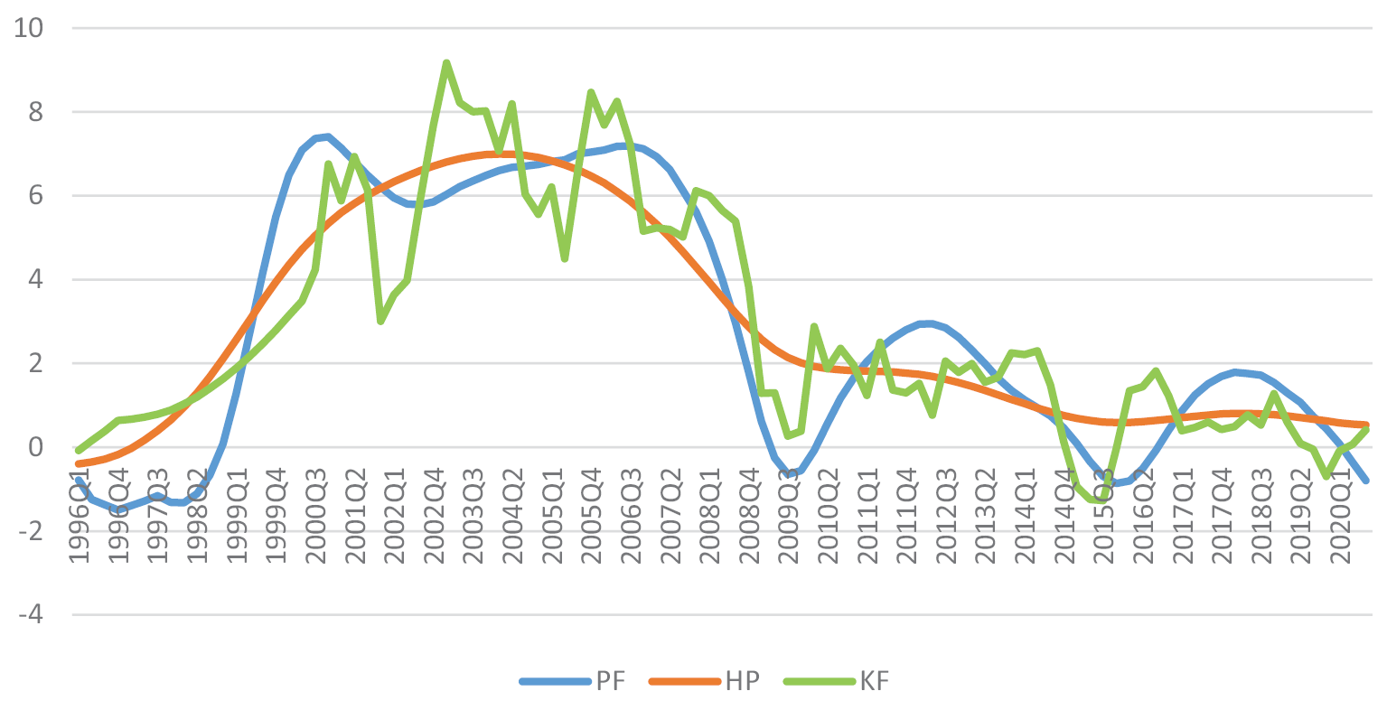
Fig. 1. Growth of Potential Output in Russia as Annual Change in %
Source: Own estimates
Similarly, looking at the growth of potential output across the three selected methods, we could observe that the shown pattern is relatively alike. Yet, the differences in results arise from different methods used in the estimation – from purely statistical filtering represented by the HP filter until the one-sided structural estimation represented by the Kalman filter.
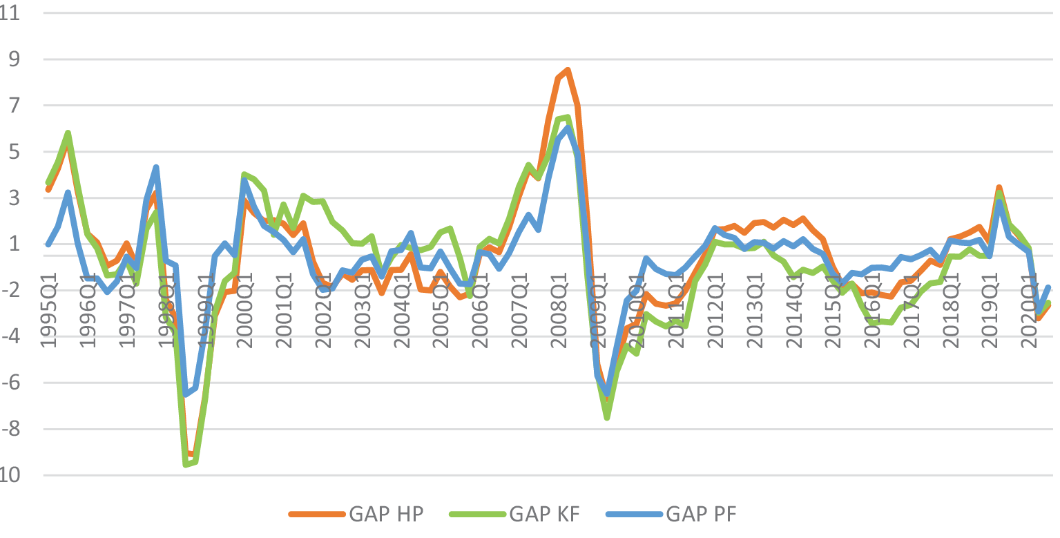
Fig. 2. Output Gap Estimates for Russia in % of Potential Output
Source: Own estimates
The individual estimates have demonstrated what is partially known from previous research on the potential output and the output gap for the other economies: the results may differ according to the methodology used. These differences are caused by different features of the used methods - as described earlier. In other words, the results are never identical, but rather approximate ones. The most volatile, in terms of output gap estimates, is the Kalman filter, while other methods have shown similar patterns. This may be, however, caused by the specific character of the filter as it considers structural variables in the country and therefore, may tend to be wavier than other methods. The results received using the Kalman filter are relatively consistent with those introduced by (Zubarev & Trunin, 2017) who present a negative output gap of around 2% in 2015.
Looking at Figure 2 we see, for instance, that the output gap estimated by the production function method in the time span of 1997Q3 until 2001Q1 recorded the lowest values, while for the period of 2005Q3 – 2008Q1, the highest. From this, we may deduce that also for the Russian Federation the potential output may not be clear-cut, and we still need to bear in mind that it is an unobservable variable. The following table presents a comparison with the OECD calculations for selected points in time.
Table 2. Output Gap: Own Estimates vs. OECD Estimates in %
|
Output gap |
1999Q1 |
2003Q1 |
2009Q2 |
2012Q4 |
2015Q4 |
2020Q3 |
|
HP filter |
-6.1 |
-0.6 |
-6.2 |
1.0 |
-1.6 |
-1.4 |
|
PF |
-3.3 |
-0.2 |
-6.0 |
0.3 |
-0.8 |
-2.1 |
|
Kalman filter |
-6.2 |
0.5 |
-7.0 |
0.3 |
-2.2 |
-2.0 |
|
OECD |
-4.8 |
0.2 |
-3.9 |
-0.4 |
-0.2 |
-2.0 |
Source: Own estimates; OECD Database (2021)
6. Conclusion
This article has primarily dealt with different output gap estimates for the contemporary economy of the Russian Federation. The main motivation was the lack of coverage in this field, both in terms of international institutions and theoretical works/academic literature. Analysing Russia’s potential output by using different estimation techniques should thus partially fill in the existing gap. Given the specificities of the Russian economy, the different structure, capital endowment, capital-to-labour ratio, and quite atypical character of the past crises, the potential output of the country has been sometimes severely affected, as presented by our complex analysis. Our comparison of methodologies demonstrates what vantage point should be adopted to treat Russia’s recent economic development.
We determined that the current sluggish performance of the Russian economy largely goes back to the slowdown of the growth of potential output. More specifically, our estimates show that it reached a growth rate just between -0.1% (using the Kalman filter) and 0.6% (using Production Function) in 2019, which shows a rare consistency in the estimates. It follows that the output gap in Russia appears to have been very close to zero in 2019, suggesting the economic slack is not caused by the cyclical factors. This clearly changed in 2020 due to the outbreak of the COVID-19 related recession.
The causes of relatively poor structural growth factors are varied. The labour market starts to suffer from the lack of labour force, as the working age population (15-64) has been declining sharply since 2010. Nevertheless, this has been partially offset by decreases in both unemployment and participation rates. Capital accumulation has also eased pace since 2010, but these factors alone cannot fully explain the overall potential output figures. We deem that one of the main causes limiting the total factor productivity growth could be the still high dependency on the oil and gas reserves; therefore, the Russian economy still needs to undergo a diversification process which typically enhances the production capacity of the industrialised economies. Should not these challenges be appropriately coped with, Russia may ultimately find its potential capacity growing relatively slowly, instead of a robust and sustainable expansion – i.e., something which it may now be well positioned for.
References
Articles in journals and conference proceedings
Blanchard, O.J. & Quah, D. (1989). The Dynamic Effects of Aggregate Demand and Supply Disturbances. The American Economic Review, Vol. 79, issue 4, p. 655–673.
D’Auria, F. et al (2010). The Production Function Methodology for Calculating Potential Growth Rates and Output Gaps. European Economy, 420. doi: https://doi.org/10.2765/71437
Giorno, C., Richardson, P., Roseveare, D., & Van Den Noord, P. (1995). Estimating Potential Output, Output Gaps and Structural Budget Balances. OECD Economics Department Working Papers, Vol. 152. https://doi.org/10.1787/533876774515
Foltynova, K. (2020). Migrants Welcome: Is Russia Trying To Solve Its Demographic Crisis By Attracting Foreigners? Radio Free Europe/Radio Liberty.
Retrieved from https://www.rferl.org/a/migrants-welcome-is-russia-trying-to-solve-its-demographic-crisis-by-attracting-foreigners-/30677952.html
Hanson, P. (2009). Russia to 2020. Finmeccanica Occasional Paper, November 2009, p. 28–30.
Hodrick, R.J. & Prescott, E.C. (1997). Post-war U.S. Business Cycles: An Empirical Investigation. Journal of Money, Credit and Banking, Vol. 29, issue 1, p. 1–16. doi: https://doi.org/10.2307/2953682
Izyumov, A. & Vahaly, J. (2008). Old Capital vs. New Investment in Post-Soviet Economies: Conceptual Issues and Estimates, Comparative Economic Studies, Vol. 50, issue 1, p. 79–110. doi: https://doi.org/10.1057/palgrave.ces.8100237
Kreptsev, D. & Seleznev, S. (2018). Forecasting for the Russian Economy Using Small-Scale DSGE Models. Russian Journal of Money and Finance, Vol. 77, issue 2, p. 51–67. doi: https://doi.org/10.31477/rjmf.201802.51
Kluege, J. (2019). Russia’s economy until 2030: Falling behind, Atlantic Community.
Retrieved from https://atlantic-community.org/russias-economy-until-2030-falling-behind/
Kuboniwa, M. (2010). Diagnosing ‘Russian Disease’: Growth and Structure of the Russian Economy Then and Now, RRC Working Paper 28
Michaelides, P. & Millos, J. (2009). TFP Change, Output Gap and Inflation in the Russian Federation (1994–2006). Journal of Economics and Business, Vol. 61, issue 4, p. 339–352. https://doi.org/10.1016/j.jeconbus.2008.10.001
Mourre, G. (2009). What Explains the Differences in Income and Labour Utilisation and Drives Labour and Economic Growth in Europe? A GDP Accounting Perspective. Economic papers 354.
Oomes, D. & Dynnikova, O. (2006). The Utilization-Adjusted Output Gap: Is the Russian Economy Overheating? IMF working papers 68. https://doi.org/10.5089/9781451863284.001
Schwabe, A. (2019). An outlook on Russia’s economy: Financial strength and economic weakness. Raiffeisen Bank International 2019. Retrieved from https://emerging-europe.com/voices/an-outlook-on-russias-economy-financial-strength-and-economic-weakness/
Zubarev, A.V. & Trunin, P.V. (2017). The analysis of the dynamics of the Russian economy using the output gap indicator. Studies on Russian Economic Development, Vol. 28, issue 1, p. 126–132. https://doi.org/10.1134/S1075700717020149
Government, financial and statistical bodies
Federal Service for State Statistics (ROSSTAT) (2020). National Accounts. Retrieved from https://rosstat.gov.ru/accounts
IMF (2021). World Economic Outlook. Retrieved from https://www.imf.org/en/Publications/WEO/Issues/2021/03/23/world-economic-outlook-april-2021
Moody’s Analytics (2021). Economic Data & Forecasts. Retrieved from https://www.economy.com/products/data
OECD Database (2021). Russian Federation. Retrieved from https://data.oecd.org/russian-federation.htm#profile-economy
UN World Population Ageing 2019 (2019). Retrieved from https://www.un.org/en/development/desa/population/publications/pdf/ageing/WorldPopulationAgeing2019-Highlights.pdf
World Bank (2020). Russia Economic Report (2020). Retrieved from https://openknowledge.worldbank.org/bitstream/handle/10986/34219/Russia-Recession-and-Growth-Under-the-Shadow-of-a-Pandemic.pdf?sequence=4&isAllowed=y
World Bank (2021). World Development Indicators: Russia. Retrieved from https://databank.worldbank.org/reports.aspx?source=2&country=RUS
Worldometer (2021). Oil Production by Country. Retrieved from https://www.worldometers.info/oil/oil-production-by-country/
Worldometer (2021). Oil Reserves by Country. Retrieved from https://www.worldometers.info/oil/oil-reserves-by-country/
Appendix 1. Raw Data Used
|
|
Nominal |
Real |
Gross F. Cap. |
Unempl. |
Total |
Population |
|
bil. RUB. |
bil. 2016 RUB. |
bil. 2016 RUB. |
%. LFS. |
mil. persons. |
mil. |
|
|
|
Nominal |
Real |
Gross F. Cap. |
Unempl. |
Total |
Population |
|
bil. RUB. |
bil. 2016 RUB. |
bil. 2016 RUB. |
%. LFS. |
mil. persons. |
mil. |
|
|
1995Q1 |
1121.9 |
45544.9 |
8554.3 |
2.75 |
66.82 |
99.04 |
|
1995Q2 |
1433.6 |
45900.0 |
11238.5 |
3.06 |
66.85 |
99.07 |
|
1995Q3 |
1752.1 |
46428.6 |
9027.0 |
3.31 |
66.75 |
99.09 |
|
1995Q4 |
1760.8 |
45376.7 |
10566.7 |
3.50 |
66.52 |
99.13 |
|
1996Q1 |
2041.2 |
44525.6 |
8445.1 |
3.69 |
66.29 |
99.19 |
|
1996Q2 |
2137.8 |
44327.2 |
7577.9 |
3.88 |
66.06 |
99.26 |
|
1996Q3 |
2214.2 |
43873.3 |
7131.8 |
4.11 |
65.35 |
99.36 |
|
1996Q4 |
2284.0 |
43973.8 |
8349.3 |
4.37 |
64.14 |
99.46 |
|
1997Q1 |
2325.0 |
44329.3 |
7880.0 |
4.64 |
62.95 |
99.57 |
|
1997Q2 |
2509.3 |
43960.1 |
7326.8 |
4.92 |
61.76 |
99.69 |
|
1997Q3 |
2527.3 |
45120.6 |
7506.9 |
6.24 |
61.82 |
99.85 |
|
1997Q4 |
2687.8 |
45563.7 |
6717.8 |
8.50 |
63.23 |
100.03 |
|
1998Q1 |
2631.8 |
43671.8 |
7167.1 |
10.54 |
64.63 |
100.26 |
|
1998Q2 |
2730.5 |
43527.1 |
6983.1 |
12.41 |
66.01 |
100.51 |
|
1998Q3 |
2948.4 |
41139.1 |
6684.3 |
13.25 |
66.84 |
100.77 |
|
1998Q4 |
3439.1 |
41404.2 |
5333.5 |
13.12 |
67.07 |
101.02 |
|
1999Q1 |
4190.3 |
42880.9 |
6786.0 |
13.00 |
67.29 |
101.24 |
|
1999Q2 |
4792.5 |
44898.4 |
6958.1 |
12.87 |
67.51 |
101.43 |
|
1999Q3 |
5651.9 |
45854.6 |
6875.0 |
12.62 |
67.12 |
101.60 |
|
1999Q4 |
5893.5 |
46405.8 |
6544.2 |
12.21 |
66.06 |
101.76 |
|
2000Q1 |
6930.5 |
48839.0 |
7835.7 |
11.80 |
65.02 |
101.90 |
|
2000Q2 |
7310.6 |
49224.5 |
7824.6 |
11.17 |
65.26 |
102.02 |
|
2000Q3 |
8084.0 |
49731.4 |
8006.4 |
10.66 |
65.32 |
102.13 |
|
2000Q4 |
8565.6 |
50468.4 |
8099.6 |
10.28 |
65.20 |
102.23 |
|
2001Q1 |
8722.9 |
51143.2 |
8381.6 |
9.84 |
64.93 |
102.31 |
|
2001Q2 |
9218.3 |
51680.5 |
8659.2 |
9.37 |
65.09 |
102.37 |
|
2001Q3 |
9724.3 |
52763.7 |
8863.7 |
9.26 |
65.37 |
102.43 |
|
2001Q4 |
10049.5 |
52736.6 |
9000.9 |
8.97 |
65.63 |
102.47 |
|
2002Q1 |
10447.2 |
53113.2 |
8626.6 |
8.03 |
66.89 |
102.51 |
|
2002Q2 |
11235.9 |
53909.7 |
8807.7 |
8.27 |
66.74 |
102.53 |
|
2002Q3 |
13012.7 |
55154.2 |
9133.3 |
8.11 |
67.00 |
102.54 |
|
2002Q4 |
11800.8 |
55953.2 |
9291.6 |
8.55 |
66.55 |
102.53 |
|
2003Q1 |
13153.5 |
57165.4 |
9649.4 |
8.65 |
66.17 |
102.50 |
|
2003Q2 |
13678.1 |
58176.1 |
10057.2 |
8.72 |
66.17 |
102.43 |
|
2003Q3 |
13811.7 |
58612.6 |
10302.4 |
8.63 |
66.44 |
102.35 |
|
2003Q4 |
14877.9 |
60254.0 |
10758.0 |
8.28 |
67.14 |
102.25 |
|
2004Q1 |
16554.9 |
61320.7 |
11349.8 |
8.51 |
66.95 |
102.15 |
|
2004Q2 |
17350.1 |
62822.4 |
11563.6 |
8.00 |
67.65 |
102.06 |
|
2004Q3 |
17249.9 |
62931.9 |
11394.8 |
7.98 |
67.66 |
101.97 |
|
2004Q4 |
20679.1 |
63982.5 |
11862.0 |
8.17 |
67.56 |
101.89 |
|
2005Q1 |
20763.1 |
65596.8 |
12662.7 |
7.54 |
68.06 |
101.83 |
|
2005Q2 |
22021.2 |
66256.4 |
12461.9 |
7.53 |
68.29 |
101.77 |
|
2005Q3 |
22641.9 |
67011.4 |
13192.8 |
7.59 |
68.57 |
101.72 |
|
2005Q4 |
25495.9 |
68171.3 |
12796.0 |
7.37 |
69.02 |
101.66 |
|
2006Q1 |
27385.3 |
70397.8 |
13963.4 |
6.89 |
69.20 |
101.60 |
|
2006Q2 |
27658.6 |
71633.9 |
14774.2 |
7.48 |
68.78 |
101.54 |
|
2006Q3 |
29104.8 |
72474.5 |
15558.8 |
7.07 |
69.20 |
101.50 |
|
2006Q4 |
30324.5 |
74207.5 |
15519.7 |
6.78 |
69.49 |
101.49 |
|
2007Q1 |
32640.7 |
76106.9 |
16629.2 |
6.18 |
70.72 |
101.53 |
|
2007Q2 |
34719.9 |
77844.0 |
17639.3 |
6.06 |
70.68 |
101.61 |
|
2007Q3 |
36834.9 |
78360.5 |
18001.8 |
5.99 |
70.68 |
101.71 |
|
2007Q4 |
40089.5 |
81012.8 |
19684.6 |
5.77 |
71.00 |
101.82 |
|
2008Q1 |
41450.4 |
83105.6 |
20662.1 |
5.88 |
71.38 |
101.93 |
|
2008Q2 |
44010.4 |
84011.8 |
20814.0 |
5.59 |
71.40 |
102.04 |
|
2008Q3 |
44873.2 |
83379.3 |
20416.6 |
6.21 |
70.86 |
102.15 |
|
2008Q4 |
40927.7 |
79915.5 |
19481.6 |
7.15 |
70.37 |
102.27 |
|
2009Q1 |
39551.8 |
75475.8 |
17353.6 |
8.28 |
69.38 |
102.40 |
|
2009Q2 |
39793.8 |
74656.2 |
16754.3 |
8.70 |
69.19 |
102.54 |
|
2009Q3 |
40672.3 |
76183.8 |
17127.9 |
8.29 |
69.39 |
102.67 |
|
2009Q4 |
41562.3 |
77836.0 |
17797.7 |
7.93 |
69.68 |
102.78 |
|
2010Q1 |
46835.8 |
78345.1 |
17795.6 |
8.00 |
69.14 |
102.87 |
|
2010Q2 |
46820.0 |
79750.5 |
18296.7 |
7.50 |
69.97 |
102.93 |
|
2010Q3 |
49243.2 |
79772.9 |
18544.4 |
7.01 |
70.27 |
102.96 |
|
2010Q4 |
51693.9 |
80063.1 |
18442.2 |
6.81 |
70.36 |
102.96 |
|
2011Q1 |
55906.5 |
80506.4 |
18297.6 |
6.88 |
70.26 |
102.92 |
|
2011Q2 |
58878.8 |
81336.4 |
18939.2 |
6.56 |
70.81 |
102.82 |
|
2011Q3 |
60552.6 |
82330.0 |
19403.6 |
6.41 |
71.18 |
102.70 |
|
2011Q4 |
62845.9 |
83348.4 |
20005.2 |
6.12 |
71.18 |
102.57 |
|
2012Q1 |
64988.9 |
84599.6 |
20289.6 |
5.89 |
70.80 |
102.45 |
|
2012Q2 |
66435.8 |
84944.4 |
20468.4 |
5.46 |
71.89 |
102.31 |
|
2012Q3 |
67423.4 |
85382.4 |
20850.4 |
5.31 |
71.76 |
102.16 |
|
2012Q4 |
68516.4 |
85439.6 |
20786.8 |
5.14 |
71.73 |
101.98 |
|
2013Q1 |
69242.6 |
86072.4 |
21063.6 |
5.44 |
71.58 |
101.77 |
|
2013Q2 |
70026.0 |
86365.6 |
21148.8 |
5.47 |
71.38 |
101.58 |
|
2013Q3 |
71654.2 |
86400.4 |
21045.6 |
5.52 |
71.26 |
101.44 |
|
2013Q4 |
72769.3 |
86899.6 |
20924.0 |
5.48 |
71.36 |
101.43 |
|
2014Q1 |
74742.8 |
86893.2 |
20852.0 |
5.21 |
71.47 |
101.56 |
|
2014Q2 |
78888.0 |
87312.0 |
20814.8 |
5.09 |
71.50 |
101.77 |
|
2014Q3 |
79843.3 |
87034.4 |
20566.4 |
5.14 |
71.45 |
101.97 |
|
2014Q4 |
81468.2 |
86829.2 |
20146.8 |
5.20 |
71.67 |
102.07 |
|
2015Q1 |
81788.4 |
85945.2 |
19626.4 |
5.43 |
72.25 |
102.00 |
|
2015Q2 |
81994.1 |
85369.2 |
18612.8 |
5.61 |
72.30 |
101.79 |
|
2015Q3 |
84718.6 |
85534.4 |
18151.6 |
5.52 |
72.43 |
101.51 |
|
2015Q4 |
85254.4 |
85314.0 |
17915.6 |
5.72 |
72.27 |
101.21 |
|
2016Q1 |
83350.4 |
85476.0 |
17767.6 |
5.63 |
72.08 |
100.97 |
|
2016Q2 |
84810.6 |
85522.0 |
18237.6 |
5.70 |
72.33 |
100.76 |
|
2016Q3 |
86022.4 |
85608.4 |
18612.8 |
5.48 |
72.60 |
100.57 |
|
2016Q4 |
87833.2 |
86301.6 |
19223.6 |
5.34 |
72.54 |
100.39 |
|
2017Q1 |
90809.4 |
86530.4 |
19324.4 |
5.33 |
72.19 |
100.21 |
|
2017Q2 |
90750.6 |
87069.2 |
19882.0 |
5.24 |
72.05 |
100.02 |
|
2017Q3 |
91913.9 |
87632.4 |
19367.6 |
5.23 |
72.08 |
99.82 |
|
2017Q4 |
93596.3 |
87653.2 |
19874.8 |
5.04 |
72.24 |
99.62 |
|
2018Q1 |
100775.2 |
88814.4 |
20050.0 |
4.88 |
72.49 |
99.43 |
|
2018Q2 |
104447.5 |
89086.0 |
19384.8 |
4.81 |
72.47 |
99.24 |
|
2018Q3 |
106612.6 |
89413.6 |
20257.2 |
4.78 |
72.31 |
99.05 |
|
2018Q4 |
106134.1 |
89798.4 |
19472.8 |
4.76 |
72.15 |
98.86 |
|
2019Q1 |
109965.2 |
89375.2 |
19615.2 |
4.66 |
71.84 |
98.68 |
|
2019Q2 |
109402.6 |
91620.0 |
20318.8 |
4.62 |
71.65 |
98.50 |
|
2019Q3 |
111903.7 |
90332.0 |
20165.6 |
4.58 |
71.62 |
98.31 |
|
2019Q4 |
108938.1 |
90025.2 |
20327.2 |
4.55 |
71.94 |
98.11 |
|
2020Q1 |
111573.0 |
89595.6 |
19154.8 |
4.48 |
71.72 |
97.90 |
|
2020Q2 |
96492.0 |
87058.0 |
17372.4 |
6.06 |
70.19 |
97.67 |
|
2020Q3 |
108281.3 |
87664.4 |
15539.2 |
6.57 |
69.85 |
97.45 |