Ekonomika ISSN 1392-1258 eISSN 2424-6166
2021, vol. 100(2), pp. 101–132 DOI: https://doi.org/10.15388/Ekon.2021.100.2.5
Evaluation of Stackelberg Leader-Follower Interaction Between Policymakers in Small-Scale Open Economies*
Metin Tetik
Faculty of Applied Sciences, Uşak University, Turkey
E-mail: metin.tetik@usak.edu.tr
Reşat Ceylan
Faculty of Economics and Administrative Sciences, Pamukkale University, Turkey
E-mail: rceylan@pau.edu.tr
Abstract. The problem of coordination between policymakers seems to have created fundamental problems related to economic and social costs, targeted inflation, potential growth, and a high budget deficit. To resolve these problems in this framework, it is important to see the results of the interaction between policymakers and to propose an optimal policy strategy. In this study, the interactions between monetary and fiscal policymakers are examined game theoretically within the framework of the New Keynesian model. The strategic interaction between these policymakers is assessed using the DSGE (Dynamic Stochastic General Equilibrium) model for a small open economy. From this point of view, the interaction between policymakers is assessed within the framework of hypothetical scenarios. The optimal monetary and fiscal policies for a small open economy are derived from the leader-follower mechanism solution known as the Stackelberg solution. Optimal Stackelberg policy rules derived for a small open economy contribute to the literature of economics. The performance of the game theoretically derived optimal policy rules is evaluated through dynamic simulation within the framework of counterfactual experiments. The parameters developed for the model are calibrated for the Turkish economy. Dynamic simulation of the models, the impulse response functions, and the social loss analysis shows that the optimal policy mix for the Turkish economy is when the monetary policymaker is the leader, and the fiscal policymaker is the follower.
Keywords: New Keynesian Model, Dynamic Stochastic General Equilibrium Model, Game Theory, Stackelberg Solution
_________
* This study, Metin Tetik’s Pamukkale University Institute of Social Sciences, Economics Department at acceptable Ph.D. Thesis “A Game Theoretical Approach to the Interaction Between Monetary and Fiscal Policies In The New Keynesian Model Framework: The Case Of Turkey” is made from his work.
Received: 22/02/2021. Revised: 19/05/2021. Accepted: 25/05/2021
Copyright © 2021 Metin Tetik, Reşat Ceylan. Published by Vilnius University Press
This is an Open Access article distributed under the terms of the Creative Commons Attribution License, which permits unrestricted use, distribution, and reproduction in any medium, provided the original author and source are credited.
1. Introduction
In traditional macroeconomics literature macroeconomic policies are formed by the behavior of policymakers. Macroeconomic policies are implemented by the monetary and fiscal policymakers whose objectives can sometimes conflict and whose effects are strong. These policymakers determine and apply the optimal policy rule to shape the structure of the economy and achieve their objectives. The different objectives of the policies implemented by the policymakers and their conflicting objectives make the optimal policy rules co-dependent and affect the macroeconomic policy formation process. Due to the interaction of policymakers in the formation process of macroeconomic policies, it becomes crucial to model this process within the framework of game theory to better establish this interaction. In game theoretical macroeconomic policy models, policymakers are defined units that have objectives and preferences and try to maximize their benefit and minimize their loss, as is the case with economic actors such as households and firms. In these models, policies take into account the mutual strategic interaction between policymakers. Therefore, it can be said that policymakers are considered as units (players) with individual objectives, expectations, and preferences in a game theoretical framework. Game theoretical policy models, which were put forward as a result of the new political economy approach, became a research field that brought together political and economic behavior in the 1980s. Compared to the past, methods such as game theory and econometrics used by the new political economy approach enabled a better understanding and a more detailed assessment of the interaction between economic and political behavior of economic units (Telatar and Erdoğan, 1997).
When examining the policy objectives of monetary and fiscal policymakers one can observe that they may tend to develop policy preferences that are far from cooperation. For example, from the fiscal policymaker’s (government) perspective, voters’ desire for lower tax rates and higher transfer spendings can lead the government to adopt an expansionary policy if inflation is in line with expectations in the short run. The monetary policymaker, on the other hand, thinks that inflation is a bigger problem since he views the economy from a long-term perspective. Therefore, policymakers may adopt opposing policy preferences (Blinder, 1983).
Bartolomeo and Gioacchino (2004) signify the decisions of policymakers as a policy mix. According to this study, these policy mixes can be deemed as four different strategic moves. In the first policy mix, monetary and fiscal policymakers act simultaneously. In the second, the monetary policymaker has the first-mover advantage, and the fiscal policymaker follows this move. In the third policy mix, the monetary policymaker responds by the budget decisions of the fiscal policymaker and the fiscal needs of the state which makes it the follower. In the last policy mix, both policymakers try to claim the leader position. In the game-theoretical approach to monetary and fiscal policy, policy authorities determine their strategies as leaders or followers and form policies accordingly.
If both policymakers act as followers, then the solution will be achieved by Nash equilibrium in the form of a two-stage game where players make their decisions simultaneously without knowing the move of the opponent. The Nash equilibrium here may be far from being an equilibrium that minimizes social loss. Nordhaus (1994) showed that the situation where policy authorities act without cooperation based on their response functions is an equilibrium in which both policymakers are unhappy, similar to Nash equilibrium. This is the case with high interest rates and budget deficits which are desired by neither policymaker because the best move of fiscal policymaker which is to reduce unemployment and increase spending (budget deficit situation) is countered by high interest rates applied by the fiscal policymaker to keep inflation under control. Therefore, it can be said that this is an example of “the prisoners dilemma” which is a popular game in game theory literature (Tetik and Ceylan, 2017).
When we look at the interaction between policymakers within the framework of the Stackelberg approach, if a policymaker acts as a leader, then the solution will occur when the follower chooses the optimal policy for himself and the leader will create the optimal policy by considering the behavior of the follower. But if both policymakers act as leaders, the solution is often called warfare, and this represents a non-cooperative game. From this point of view, acting as leader-follower can be considered a suitable strategy for policymakers. What is meant by leadership here is the difference in policy response and implementation times and decision-making processes. In this case, it becomes crucial to determine which player should move first.
As a result, the contribution of this study can be summarized as follows. First, the study makes a new contribution to the literature with the game-theoretical analysis of the leader-follower setting between the monetary and fiscal policies we have developed for the small-scale open economy. Secondly, thorough policy analysis in the framework of counterfactual experiments has not been previously performed for the Turkish economy. With this information in mind, the rest of the study is organized as follows. The second section presents the related literature. The third section introduces the small-scale open economy and the dynamic equations that describe it and then discusses the interaction between policymakers within the framework of game theory. Moreover, the interaction between policymakers in small open economies is assessed as the Stackelberg leader-follower game and alternative monetary and fiscal policy rules are derived for the situation in this scenario. In the fourth section, numerical analysis of game theoretically derived models is introduced. In this context, the parameters of the DSGE model are calibrated taking into account the data from the Turkish economy in the 2006:01 - 2019:12 period, and each scenario is analyzed through dynamic simulation. In the framework of counterfactual experiments, utilizing the impulse-response and social loss analysis obtained with dynamic simulation, the policy mix that would result from the least social loss for the Turkish economy is investigated. Concluding remarks and policy suggestions are presented in the fifth section.
2. Related Literature
There are studies in the literature addressing the behavior of monetary and fiscal policymakers within the game-theoretical framework. For example, Nordhaus (1994) examined the interaction between monetary and fiscal policies within the game theoretical framework in terms of independence and coordination. The policy interaction, which is examined analytically, was then evaluated employing impulse-response analysis for the US economy, using the VAR model and simulation technique. As a result of the VAR model, it has been determined that the monetary policy does not react to the fiscal policy, while the fiscal policy is positively associated with the interest rate and thus reacts to the monetary policy. According to the simulation results, it was stated that the monetary authority could not equilibrate the fiscal policy in the short term and should overreact to this. It has been demonstrated that poorly timed contractionary fiscal policies may increase unemployment in the short term, moreover, if the monetary policymaker is not cooperative, this policy will not have an effect on reducing the budget deficit and will also reduce consumption. In the light of this information, Nordhaus (1994) emphasizes the importance of policy coordination. Van Aarle et al. (1995) examined the strategic relationship between monetary and fiscal policy within the framework of debt stabilization. Taking account of the open-loop Nash and Stackelberg equilibrium Van Aarle et al. (1995) put forward the conclusion that the central bank should adopt a more independent policy. Henry et al. (1999) examine the need for monetary policymakers to adjust policy to ensure low inflation within the framework of the structure of coordination between policymakers and the independence of the central bank. The structure of coordination between policymakers is first discussed game theoretically and then empirically for the UK economy. According to the findings of the study, the increasing importance given to inflation deviation decreases the inflationary effect. Shocks create instability when there is no coordination between policymakers. The reason for this is described as a conflict of policy objectives. Important results are obtained from the solutions developed for cooperative and non-cooperative (Nash) situations. It was stated that the expansionary fiscal policy in the non-cooperative situation caused high-interest rates and created problems in combating inflation. The reason for this was explained as the central bank had to increase the interest rates abnormally to control inflation. Also, it is stated that high-interest rates cause a decrease in output. It is emphasized that, in the case of cooperation, inflation can be reduced with less effect on output. Therefore, it is stressed that the lack of cooperation between policies causes a lower growth rate, overvalued exchange rate, and a decrease in foreign trade. On the other hand, Neck (1999) examined the dynamic game model between Austrian economic data and monetary and fiscal policy. It is reported that there are only minor differences in the models predicted for cooperative and non-cooperative solutions. In addition, it is concluded that the role of the government in terms of macroeconomic objectives is bigger than the central bank. Buti et al. (2001) analyze the interaction between the central bank and the fiscal authority as a simple game. They assert that the complementarity or substitutability of policymakers depends largely on the type of shock affecting the economy. If the government implements a policy to increase output above its natural level, there is an output gap deviation in the non-cooperation situation. However, both ‘output gap deviation’ and ‘inflation divergence’ are encountered in the case of cooperation. Besides, these deviations will disappear if the government only maintains cyclical stability. Van Aarle et al. (2002) set up different dynamic game scenarios to examine the effects of cooperation between policymakers in EMU. These scenarios are (i) non-cooperative monetary and fiscal policies, (ii) partial cooperation, and (iii) full cooperation in symmetrical and asymmetrical settings that differ according to the structural characteristics of countries, policy preferences, and/or bargaining power. Dynamic simulation technique was used to evaluate these scenarios. Consequently, the effects of the sustainability of a given coalition and optimal strategies and the results of macroeconomic adjustment are highly sensitive to initial calibrations of preferences and structural model parameters. Cooperation is often effective for the fiscal policymaker. The non-cooperative Nash equilibrium occurs when the assumptions for countries in the European Monetary Union are asymmetrical. In most simulations, full cooperation does not provide Pareto improvement for the ECB. Situations in which the ECB cooperates with one government against another generally do not produce policies that improve stability in monetary and fiscal policies. Another study on this subject is by Lambertini and Rovelli (2003), in which they theoretically examine the relationship between monetary and fiscal policy in terms of macroeconomic stability. The model is analyzed in terms of aggregate demand (AD) and aggregate supply (AS) for a closed simple economy. The findings have shown that the Stackelberg solution is preferable to the Nash solution. Kirsanova et al. (2005) examined the interaction between monetary and fiscal policies within the framework of reactions against economic shocks in a dynamic structure. In the paper, the situation in which both policymakers are optimistic is assessed firstly and the best result in terms of social loss has been achieved. What we mean by optimism here is that the fiscal authority determines almost all the burden according to the objective of the monetary authority in terms of macroeconomic stability. Secondly, if the monetary authority is optimistic but the fiscal authority deviates from the objective, the greatest social loss in terms of Nash equilibrium occurs. In this case, if each authority tries to achieve economic stability with one-sided individual effort, a rapid accumulation of public debt occurs. Thirdly, if the monetary authority is optimistic, fiscal authority deviates from the target, and fiscal authority becomes the leader, the result is almost as good as if both policymakers were optimistic. Fragetta and Kirsanova (2010) analyzed the interaction between a monetary and fiscal policy with the Bayesian estimation method using a small open economy model on data from United Kingdom, United States, and Sweden. In the study, it was assumed that monetary and fiscal authorities strategically behave as in non-cooperative policy games and different leadership regimes were compared. It is concluded that, according to micro-founded social preferences, fiscal leadership policy is the most appropriate model for the UK and Sweden, while for the United States Nash or non-cooperative regime is the most appropriate model. Saulo et al. (2013) analyzed the interaction between a monetary and fiscal policy with Brazilian data within the framework of game theory. In the model where they derived and analyzed the Nash and Stackelberg solutions for a small closed economy, it was found that the lowest social loss occurs when the monetary authority is the leader.
Some studies on the interaction between monetary and fiscal policies are based on an examination of the structure of policy interaction in certain countries. In this context, it is seen that the decisions of policymakers affect not only their objectives but also that of the other policymaker, positively or negatively. Other studies in the literature are on how effective policy coordination can be ensured. It is seen that effective coordination varies in different studies due to the structure of theoretical models and the variation of these models according to the countries. In this study, based on the New Keynesian macroeconomic model, alternative policy interactions for a small open economy are game theoretically examined. In this framework, behaviors of policymakers are modeled according to alternative leader-follower scenarios. Giannoni and Woodford (2002a), Giannoni and Woodford (2002b) were consulted for the solution of models, and Saulo et al. (2013) for game-theoretical setting.
3. Representative Economy: Small-Scale Open Economy
In this study, the representative economy needed to derive policy rules based on the strategic interaction of monetary and fiscal policymakers is formed based on small-scale open economy models described in Gali and Monacelli, (2005) and (2015) and Çebi (2012). Our intuition for choosing this model is that it contains an open economy setup, unlike Saulo et al. (2013), which inspired us. Besides, the model’s factoring of Calvo style nominal price rigidities, distortionary taxation, rule of thumb price-setters, and perfect exchange rate pass-through properties was also effective. In this model, it is assumed that domestic policy decisions for each economy do not have any impact on the rest of the world. Also, when different economies are exposed to associated shocks, it is assumed that they share the same preferences, technology, and market structure. Such an economy consists of resident households and firms in monopolistic competition, and the two policymakers, namely the government and the central bank.
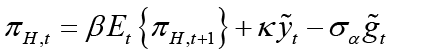
The New Keynesian Phillips curve for the open small economy is represented as follows:
 (1)
(1)
In Equation 1 πH,t represents the domestic inflation which shows the rate of change in the domestic goods prices index, that is, the CPI inflation.  represents the domestic expected inflation.
  is the domestic output gap. The domestic output gap (
 ) is defined as the deviation of domestic output(log)(yt) from its natural level
  , thus (
 ).
).  is defined as fiscal deficit and indicates the gap between the fiscal policy variable
  and its optimal value in the absence of nominal rigidities (
 ). In the equation parameter κ is expressed as the slope of the New Keynesian Phillips curve.1
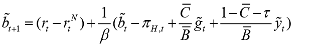
The dynamic IS equation for the open small economy in terms of output gap is obtained as follows:
 (2)
(2)
In equation 2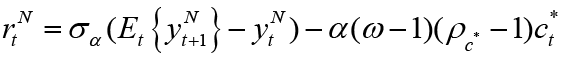 is the nominal natural interest rate. It is also possible to show the interest rate in terms of the natural productivity level (at) and world output shocks (ct* ) if we change the potential output2:

Here, the natural productivity level and world output shocks are exogenously determined and both variables are assumed to follow an autoregressive (AR (1)) process with one lag.
Government spending and taxes are assumed to be zero in a flexible price economy. This means that there is no budget deficit or surplus in flexible price equilibrium. Cebi (2012), Fragetta and Kirsanova (2010) assume that natural level of inflation and government spending also has equal to the zero, that is,  . Hence it can be expressed as
  and
and  .
.
The interaction between monetary and fiscal policies stems mainly from the government’s intertemporal budget constraint. The fiscal policy move, which may cause an increase in the current budget deficit, will be financed by an increase in future tax revenues or the value of so-called nominal government obligations, such as money. This is referred to as “The Unpleasant Monetarist Arithmetic” of Sargent and Wallace (1981). Hence, the hypothetical model used in this study is complemented by a fiscal constraint. Fragetta and Kirsanova (2010) express the linearized government debt payment restriction (fiscal restriction) as follows3:
 (3)
(3)
In equation 3, 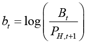 where B is nominal debt stock.
  and
and  represent steady state debt/GDP ratio and steady state consumption/GDP ratio respectively. τ is the fixed income tax rate.
The limits of the hypothetical economy needed for game-theoretical modeling of the strategic interaction between monetary and fiscal policymakers are illustrated by equations 1, 2, and 3 which represent a small open economy based on New Keynesian macroeconomic theory. The optimal policy rules (strategies) of monetary and fiscal policymakers are derived based on these equations.
3.1 Derivation of the Stackelberg Optimal Interest Rate and Spending Rule
In this section, optimal response functions for each policymaker are derived depending on the nature of the leader-follower interaction between monetary and fiscal policymakers. For this, firstly, the model in which monetary and fiscal policymakers act simultaneously is considered. The policy rules derived from here are Nash equilibrium solutions. Nash equilibrium solutions are required to obtain Stackelberg equilibrium solutions because the obtained Nash equilibrium solutions also represent the optimal behavior of the follower. The objectives of monetary and fiscal policymakers are to minimize the loss functions corresponding to the equilibrium condition of the economy. Policymakers solve the optimization problem by committing to their own optimal policy rules. For the solution of optimization problems, the Lagrange technique approach is used as in the studies by Gioanni and Woodford (2001), Gioanni and Woodford (2003), and Saulo et al. (2013). This approach, which is widely used in the monetary policy literature, has been used in this study because it provides the relationship of policy rules with the desired equilibrium and time-consistent properties and remains optimal regardless of the statistical properties of the economy. 4 The solutions of the optimization problems of policymakers for each scenario obtained with the Lagrange technique approach were checked by the Maple 11 program. Before moving on to how the policy rules are derived, the objective and constraint equations of the actors in our macroeconomic model, namely monetary and fiscal policymakers, are shown in this section.
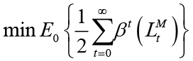
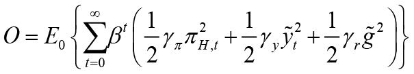
The game between monetary and fiscal policies is based on the tendency of each policymaker to minimize their social loss function. If we add the concept of time to these loss functions; we obtain: 5
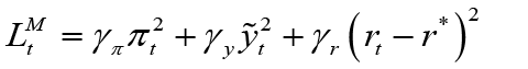
Objective function of the monetary policymaker: 6
 (4)
(4)
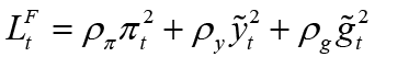
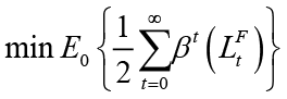
Objective function of the fiscal policymaker:
 (5)
(5)
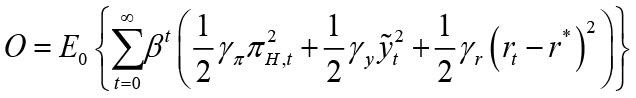
These functions represent the objective functions of both policymakers. According to the equilibrium condition of the economy in monetary and fiscal loss functions; the positive-weighted parameters γπ and ρπ represent the deviation from the inflation target, γy and ρy represent the deviation from the output gap, γr represents the deviation from the optimal interest rate and ρg represents the deviation from the optimal government spending, respectively. For the constraint equations, the aggregate supply equation in the open small economy (equation 1), aggregate demand equation (equation 2), and, finally, the government budget equation (equation 3) are used.
3.2 Stackelberg Application of the Monetary and Fiscal Policy Game
Monetary Policymaker Leadership
Suppose the monetary policymaker moves first (Stackelberg Leader). In this case, the monetary policymaker will react best by taking into account the optimal policy of its follower fiscal policymaker. The best response of the leading monetary policymaker will depend on the best response of its follower fiscal policymaker. The best response of the fiscal policymaker is the optimal policy resulting from the Nash equilibrium solution. The monetary policymaker represented as the central bank is trying to minimize the loss function 4 below 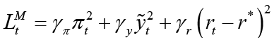 in the current period. When the monetary policymaker is the leader, the follower is the fiscal policymaker. Therefore, we need to derive the optimal policy rule of the follower. This corresponds to the best response (
 ) of the fiscal policymaker in the sub-game in the dynamic game system. In the subgame, the fiscal policymaker aims to minimize equation 5
 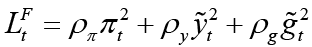 which is the loss function corresponding to the equilibrium condition of the economy. That is, in the sub-game, the fiscal policymaker solves the problem
 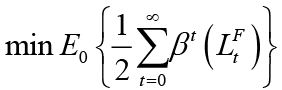 by taking into account the constraints in the economy, and thus the non-cooperative optimal nominal spending rule is the best response of the follower fiscal policymaker in the sub-game7.
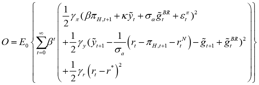
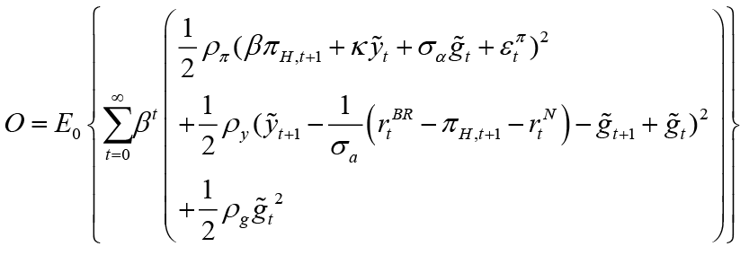
In the next stage, the aim of the monetary policymaker is to solve the following problem in part 1 of the game, considering the constraints in the economy and anticipating the best response  of the fiscal policymaker to each of her moves.8
This model has been turned into a problem represented by the objective function O in the form of unconstrained optimization. Therefore, by solving problem O, the optimal interest rate rule ( ) is obtained when the monetary policymaker is the leader:
By substituting the main equations and the policy rule of the follower (fiscal policymaker) in the objective function O, the following minimization problem is obtained:
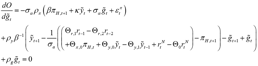
Then, the first-degree condition is obtained according to the policy target variable of leading monetary policymaker.

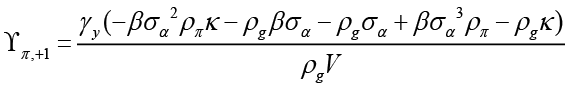
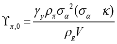
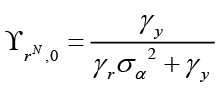
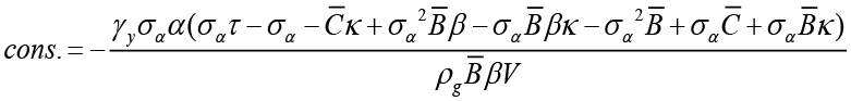
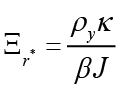
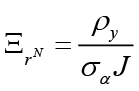
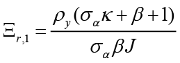
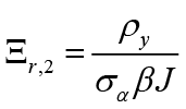
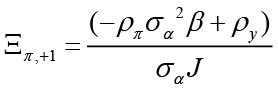
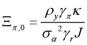
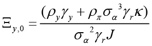
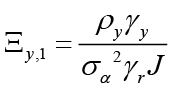
In this case, as a result of the necessary substitution and unbundling process, the optimal interest rate rule is obtained as follows when the monetary policymaker is the leader 9;

(6)
In equation 8, 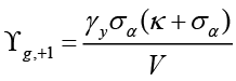 ,
,  ,
,  ,
,  ,
,  ,
,  ,
,  ,
,  ,
,  and finally
 .
.
Here,  is what we use for simplification.
Equation 6 is the interest rate rule that the monetary policymaker commits to follow when leading, and this rule depends on expected and current inflation, expected, current and past output gap, past and expected government spending and finally the equilibrium and natural interest rate. Unlike the interest rate rule obtained in the non-cooperative Nash game, this policy rule also has responses to government spending and the natural interest rate, which are other policy tools. Besides, all parameters refer to the sensitivity of interest rate (where monetary policymaker is the Stackelberg leader) to independent variables.
Fiscal Policymaker Leadership
The fiscal policymaker represented as the government tries to minimize the loss function 5, that is 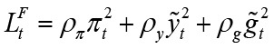 . This time, the case where the fiscal policymaker is the leader and the monetary policymaker is the follower is discussed. Therefore, we need to derive the optimal policy rule of the follower again. The optimal policy rule expressing the best policy response corresponds to the best response (
 ) of the monetary policymaker in the subgame. In the subgame, the monetary policymaker aims to minimize the monetary loss function 4
 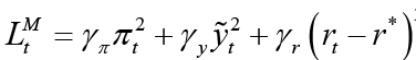 , which corresponds to the equilibrium condition of the economy. That is, in the sub-game, the monetary policymaker solves the problem
 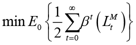 by taking into account the constraints in the economy, and therefore the non-cooperative optimal interest rule is the best response of the follower monetary policymaker in the sub-game10.

In the next stage, the aim of the fiscal policymaker is to solve the following problem in part 1 of the game, taking into account the constraints in the economy and anticipating the best response of the monetary policymaker to each move. 11
This model has been turned into a problem represented by the objective function O below in the form of unconstrained optimization, and by solving this problem, the optimal spending rule ( ) is obtained when the fiscal policymaker is the leader:
By substituting the main equations and the policy rule of the follower (monetary policymaker) in the objective function O, the following minimization problem is obtained:
Then, the first rank condition is obtained according to the policy target variable of leading fiscal policymaker.
In this case, as a result of the necessary replacement and unbundling process, the optimal interest rate rule is obtained as follows when the fiscal policymaker is the leader 12;

 (7)
(7)
In equation 9, 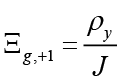 ,
,  ,
,  ,
,  ,
,  ,
,  ,
,  ,
,  ,
,  ,
,  and finally
 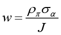 . Here we use
 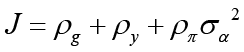 for simplification.
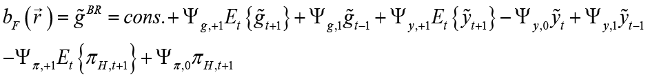
Equation 7 is the spending rule that the fiscal policymaker commits to follow when it is the leader, and this rule is based on expected and current inflation, expected, current and past output gap, expected government spending, equilibrium to supply shocks, natural and past interest rates. Unlike the spending rule obtained in the non-cooperative Nash game, this policy rule also has responses to interest rates. Also, all parameters refer to the sensitivity of government spending (where fiscal policymaker is the Stackelberg leader) to independent variables.
4. Application of Alternative Scenarios: Dynamic Simulation
In this section, a stochastic simulation of the model derived for alternative scenarios among policymakers is made. This simulation is performed to evaluate the performance of optimal monetary and fiscal policies derived for each scenario. As a result of the simulation, the effects of each scenario on social loss are analyzed by looking at their responses to exogenous shocks through impulse response functions. Loss analysis is then made to find out which scenario results in the lowest social loss.
The performance of optimal monetary and fiscal policies obtained for alternative scenarios is evaluated by a simulation using dynamic IS curve equation, New Keynesian Phillips curve equation, government budget constraint equation, and optimal monetary and fiscal policy rules. For this, the model must be calibrated. In the calibration process performance of the Turkish economy in the period 2006: 01-2019: 12 was taken into account. Thus, the computational parameters in the model were calibrated based on the values from the Turkish economy from 2006: 01-2019: 12 period. Other parameters in the model were calibrated using previous studies. Calibrated values are shown in Table 1.
Table 1. Calibration Values
|
Parameter |
Definition |
Value |
|
θ |
Domestic price stickiness degree |
0.5 |
|
σ |
Inverse elasticity of consumption substitution between periods |
3 |
|
α |
Openness degree |
0.27 |
|
φ |
Inverse elasticity of labor supply |
2 |
|
β |
Discount factor |
0.99 |
|
σa |
Standard deviation of technological innovation |
1 |
|
ρa |
AR coefficient of technology |
0.8 |
|
ρc* |
AR coefficient of foreign consumption |
0.8 |
|
γπ |
The parameter of deviation from the inflation target according to the equilibrium condition of the economy in monetary loss function |
1 |
|
ρπ |
The parameter of deviation from the inflation target according to the equilibrium condition of the economy in the fiscal loss function |
0.5 |
|
γy |
The parameter of deviation from the potential level of output according to the equilibrium condition of the economy in the monetary loss function |
0.4 |
|
ρy |
The parameter of deviation from the potential level of output according to the equilibrium condition of the economy in the fiscal loss function |
1 |
|
γr |
The parameter of deviation from the equilibrium interest rate according to the equilibrium condition of the economy in the monetary loss function |
0.5 |
|
ρg |
Parameter of deviation from equilibrium government spending (or fiscal deficit) according to the equilibrium condition of the economy in the fiscal loss function |
0.2 |
Since prominent average duration of price contracts in the literature is six months, the Calvo parameter was used as 0.50 for domestic price stickiness. The parameter value of the inverse elasticity of the substitution of consumption between periods was used as 3 as in Çebi (2012). This means that the substitution elasticity in consumption is 0.33 (1/3). The degree of openness was determined as 0.25, as in Çebi (2012), taking into account the ratio of average imports to GDP, between 2006: 01-2019: 12. On the other hand, with a similar calculation, the steady state debt / GDP ratio  was determined 0.21, and the steady state consumption / GDP ratio
  was determined 0.62, between the same periods. Fixed income tax rate, on the other hand, is determined by taking into account the tariff used in the taxation of income subject to income tax included in Article 103 of the Income Tax Code. This tariff does not change according to years, it only changes according to income categories. In the study, income tax rate was used as a fixed 0.2425 which is the average of the rates for different categories of income. The discount factor β is set at 0.99 since the annual steady state real interest rate is taken as 4%. Based on the study of Lubik and Schorfheide (2007), elasticity of substitution between domestic and foreign goods β and the elasticity of substitution between goods produced in different countries was determined as 1. This way, the coefficients ω and λ were obtained and σa = 1 determined as in Çebi (2012). In monetary and fiscal loss functions, inflation, output, optimal interest rate and deviation parameters from government spending according to the equilibrium condition of the economy were determined according to the studies of Fragetta and Kirsanova (2010), Çebi (2012), Flotho (2012) and Saulo et al (2013). In the monetary loss function, according to the equilibrium condition of the economy, the deviation from the inflation target parameter is determined as 1, the deviation parameter from the potential level of output is 0.4 and the deviation from the equilibrium interest rate parameter is 0.5. In the fiscal loss function, the deviation from the inflation target parameter is 0.5, the deviation from the potential level of output is 1 and the deviation from the equilibrium government spending parameter is 0.2, according to the equilibrium condition of the economy.
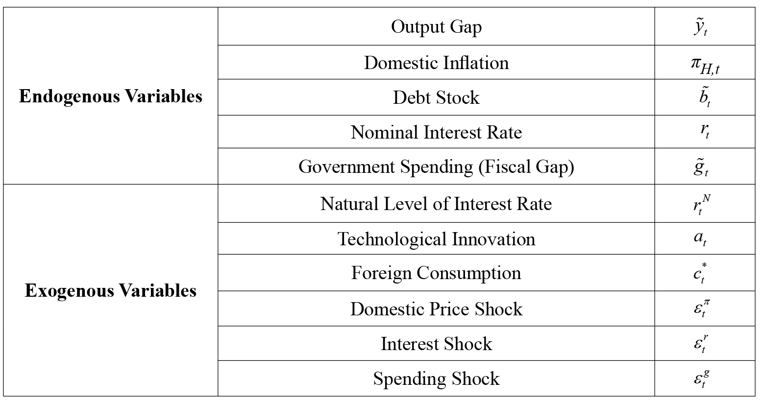
Endogenous variables in the general equilibrium model are defined as variables based on data. Exogenous variables, i.e., shock variables, are variables that express shocks that are not caused by the endogenous dynamics of the economy. In this framework, the variables in the general equilibrium model are summarized in Table 2.
Endogenous variables used in the model are the natural level of interest rate, technological innovation, foreign consumption, domestic, price shock, interest shock, and spending shock. Exogenous variables are the natural level of interest rate, technological innovation, foreign consumption, domestic price shock, interest shock, and spending shock. Among these shocks, domestic price, interest, and spending shocks reveal the real changes for the relevant period aftershocks given to data-based variables. However, the natural level of interest rate, technological innovation, and exogenous world consumption refer to shocks that are not caused by the endogenous dynamics of the economy.
Table 2. Definitions of Variables
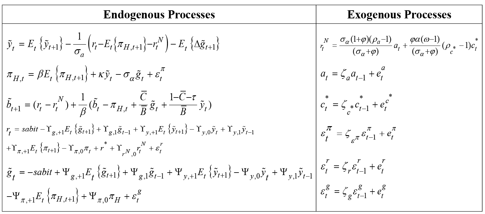
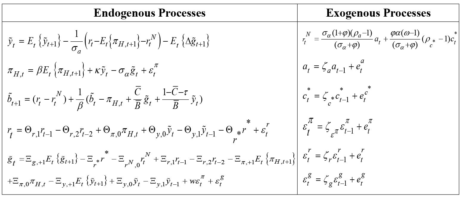
In the general equilibrium model within the framework of the Stackelberg game in which the monetary policymaker is considered as the leader, the endogenous processes again include the dynamic IS equation, the New Keynesian Phillips curve, and the government debt payment constraint equations. However, interest and spending rules consist of equations obtained as a result of the scenario where the monetary policymaker is the leader, and the fiscal policymaker is the follower. In the New Keynesian Phillips curve, shock variables are added to the policy rules of interest and spending exogenously. Exogenous processes are natural interest rate, technology defined as AR (1) process, and foreign consumption. The general equilibrium of the economy, the equations representing the open economy model, and the policy rules obtained in game theory for this scenario are shown in Table 3.
Table 3. General Dynamic Equilibrium Model in Monetary Policymaker Leadership
The general equilibrium model within the framework of the Stackelberg game in which the fiscal policymaker is considered as the leader is similar to the model where the monetary policymaker is the leader. However, interest and spending rules consist of equations obtained from the scenario where the fiscal policymaker is the leader, and the monetary policymaker is the follower. The general equilibrium of the economy, the equations representing the open economy model, and the policy rules obtained for this scenario game theoretically are shown in Table 4.
Table 4. General Dynamic Equilibrium Model in Fiscal Policymaker Leadership
4.1. Findings of Numerical Analysis
In this part of the study, stochastic simulation results of game theoretical models developed with counterfactual experiments are discussed. As stated before, the model dynamic IS equation consists of the New Keynesian Phillips curve equation, government debt payment constraint equation, and interest and spending policy rules derived for leader-follower scenarios. In this study, for the operation steps of each scenario, the DYNARE toolbox that runs on the MATLAB program which is developed for the prediction of Dynamic Stochastic General Equilibrium Models was used.
New Keynesian macroeconomic models generally tend to deal with the disruptive effects of exogenous shocks in an economy and its responses to shocks (Snowdon and Vane, 2005). With stochastic simulation, for each scenario based on the interaction between policymakers, the responses of output, inflation, debt stock, and interest rates to shocks in the assumed equilibrium economy are shown. The impulse-response functions here are obtained based on the calibration values of the parameters. Thus, it shows us when the effects of shocks in the economy on variables considered to be indicators of social loss started and how long they lasted. By comparing the responses of the endogenous variables to the shocks in the assumed equilibrium economy for each scenario it can be determined which scenario is more effective and the equilibrium dynamics of the obtained models can be analyzed. Based on the impact response analysis, the dynamic structure of the interaction between policymakers is also investigated. In this context, the effects of monetary policy shocks on the spending rule and the effects of fiscal policy shocks on the interest rate rule can be observed for the leader-follower scenarios between policymakers. Thus, by examining the dynamic structures of the leading follower mechanisms between policymakers, the game theoretically constructed scenarios are analyzed. In addition, the variances of the optimal paths of the variables are obtained with the stochastic simulation. Thus, the expected value of the social loss function of the economy at equilibrium is calculated for each scenario. In this way, it is examined which scenario minimizes the social loss function. Based on this, the findings give us a direction other than impulse-response analysis as to which is the optimal policy interaction.
4.2. Analysis of Structural Shocks: Impulse Response Analysis
Studies on New Keynesian DSGE models in the literature are generally based on the study of business cycle fluctuations and dynamic structures of these fluctuations with DSGE models developed by researchers (Bari and Şıklar, 2016). To explain the sources of business cycles in the economy, the transfer of various structural shocks on the economy is analyzed. These are done with impulse-response analysis. Structural shocks described in this study are supply (cost-push shocks), technology, and policy shocks.
During a negative supply shock, coordination between policymakers becomes important. If there is no coordination between policymakers, then contradictory policies may be followed. For example, the fiscal policymaker may prefer an expansionary policy to reduce the negative output gap that will occur as a result of a negative supply shock to its potential level. The monetary policymaker, on the other hand, can implement a contractionary policy to contain the high price increase caused by the negative supply shock. A positive or negative demand shock based on exogenous factors can cause inflation or deflation. Here again, coordination of monetary and fiscal policies becomes crucial. Policymakers can follow contractionary policies during a positive demand shock to reduce aggregate demand and contain inflation, while in the event of a negative demand shock, they can follow expansionary policies.
This part of the study explores how structural shocks affect the economy according to the nature of the interaction between policymakers and which leader-follower scenario among policymakers better manages this shock. Table-5 shows the results of the impulse-response analysis.
Fluctuations in business cycles and the instability created by this are due to shocks in aggregate supply and/or aggregate demand. Aggregate supply shocks are considered major changes in productivity. If the factors that cause productivity change are positive, then total production will be positively affected. Factors that affect efficiency positively and the development of new management and production techniques can be defined as positive changes in the quality of production inputs and these changes have an increasing effect on total production. In the macroeconomics literature, such shocks are called technology or productivity shocks. The real business cycle theory assumes that this technology shock is completely random. In the first two rows of Table 5, the way a technological shock affects the economy according to the structure of the interaction between policymakers is presented with the impulse response analysis results. Theoretically, a positive productivity shock has a decreasing effect on marginal costs. Inflation is expected to decrease as a result of the decrease in marginal costs. Along with this, the decrease in the natural interest rate is predicted to revive the economy. In the first row of Table 5, the responses of variables to a technology shock when the Stackelberg monetary policymaker is the leader and the fiscal policymaker is a follower can be seen. In this scenario, the technology shock reduces inflation in the economy, and it disappears completely after ten periods. When looking at the interaction between policymakers in the face of this shock, it is seen that both policymakers react with an expansionary policy. It is observed that although such a shock and policy mix has a positive effect on inflation and debt stock, it does not provide the desired output increase. In the second row of Table 5, when the Stackelberg fiscal policymaker is the leader and the monetary policymaker is a follower, the responses of the variables against the technology shock are seen. A positive productivity shock reduces inflation on marginal costs. However, this positive effect lasts for a period. The fall in the natural interest rate and the expansionary policy responses of both policymakers have a positive impact on output. However, this response is thought to be lagged due to wage/price rigidities. It is observed that expansionary policy responses cause inflation in the economy. The effects of expansionary policies disappear in the tenth period.
Table 5. Impulse Response Analysis Results
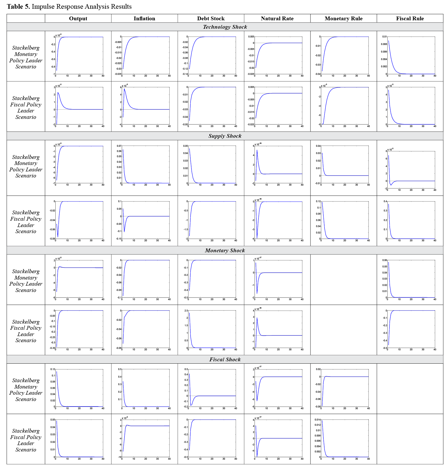
Aggregate supply shocks are known to be major changes in productivity. If the factor that causes productivity change is negative, this will affect the total production negatively. For example, factors such as an increase in energy prices, political turmoil, labor actions, government regulations that would hurt incentives, drought, earthquakes, or wars that cause an increase in costs will also negatively affect productivity and decrease the aggregate supply. In theory, cost-push shocks shift the short-run supply curve (AS) to the left by raising marginal costs. In this case, inflation rises while output decreases. With the response of monetary and fiscal policymakers to this shock, the reactions of the variables also change. In the case of negative supply shocks, the objectives of monetary and fiscal policymakers tend to conflict. While the monetary policymaker tends to implement a contractionary policy by paying attention to price stability, the fiscal policymaker can display an expansionist attitude by paying attention to output stability. In their study on the interaction between fiscal and monetary policies in Turkey, Tetik and Ceylan (2016) found that the central bank implements a contractionary monetary policy in the face of negative supply-side shocks while the fiscal authority implements an expansionary fiscal policy. Therefore, Tetik and Ceylan (2016) stated that a negative supply shock may lead to a policy conflict in Turkey. In the third and fourth rows of Table 5, the way a negative supply shock affects the economy according to the structure of the interaction between policymakers is given with the impulse response analysis results. In the third row of Table 5, the responses of the variables to a negative supply shock are seen when the Stackelberg monetary policymaker is the leader and the fiscal policymaker is the follower. In this scenario, a negative supply shock increases inflation in the economy and this effect lasts for four periods. In response to this development, the monetary policymaker implements a contractionary monetary policy. Contractionary monetary policy increases interest rates and thus decreases the output. It is observed that the fiscal policymaker has adopted a lagged contraction policy. With the effect of the policy mix in this scenario, it is seen that the debt stock gives a positive response to the negative supply shock. It is seen that the follower fiscal policymaker later reduced government spending and the debt stock decreased with increasing interest rates. With this policy mix, the economy returns to its starting position at the end of the fifth period. In the case where Stackelberg fiscal policymaker is the leader and the monetary policymaker is a follower, the responses of the variables to a negative supply shock are seen in the fourth row of Table 5. In this scenario, a negative supply shock causes inflation that lasts for one period and a decrease in output that lasts for five periods. In the face of this shock, it is seen that the fiscal policymaker has adopted an expansionary policy and gave the highest reaction compared to other scenarios. The monetary policymaker, who is a follower, exhibits the strongest contractionary policy stance compared to other scenarios. As a result of this policy mix, a deflationary situation appears to emerge.
The accordance between monetary and fiscal policy objectives and instruments is important for policy coordination. Thus, the effectiveness of an economic policy depends on the harmonious functioning of objectives and tools. Effective coordination between policymakers requires a flow of information among all actors involved in policy decision-making. A poorly executed monetary policy can prevent the implementation of a successful and effective fiscal policy, and a bad fiscal policy can prevent the implementation of a successful and effective monetary policy. For example, an overly restrictive monetary policy, whose primary objective is price stability, may cause interest rates to rise rapidly and thus threaten fiscal stability by increasing government debt repayment costs (IMF and World Bank, 2003). If price stability is not directly threatened, policymakers are not advised to take overly restrictive measures. Excessive expansionary fiscal policy behavior can also be the main reason for many economic and social problems such as high inflation, budget deficit, and low economic growth. Countries need appropriate fiscal arrangements to solve these problems. The fiscal policymaker who carries out such a policy may push the monetary policymaker to take a wrong policy attitude with excessive borrowing. Failure to take appropriate monetary policy measures as a result of lack of coordination can hurt the private sector by removing it from the credit market, and economic growth may slow down as a result of the implementation of a bad fiscal policy (Raspudic, 2012). In the fifth and sixth rows of Table 5, how a positive nominal interest rate shock (a contractionary monetary policy shock) and a positive government spending shock (expansionary fiscal policy shock) affect the economy according to the structure of the interaction between policymakers according to the impact response analysis results is seen. In the fifth row of Table 5, when the Stackelberg monetary policymaker is the leader and the fiscal policymaker is a follower, the responses of the variables to the monetary policy shock are seen. In this scenario, inflation, and output decrease with the increase in interest rates. It is seen that the fiscal policymaker, who is considered to attach importance to output stability, gave an expansionary fiscal policy response to this contractionary policy. With the effects of the expansionary fiscal policy, output increases at the end of the third period and debt returns to its initial level. In the scenario where the monetary policymaker is the leader, it is seen that the expansionary policy choice of the follower fiscal policymaker provides a non-inflationary output increase. In the sixth row of Table 5, when the fiscal policymaker of Stackelberg is the leader and the monetary policymaker is a follower, the responses of the variables to the monetary policy shock are seen. In this scenario, inflation, and output decrease with the increase in interest rates. The fiscal policymaker, whose political priority is supposed to be output increase and stability, gives an expansionary response to the contractionary policy move of the monetary policymaker in the other three scenarios. However, it appears that in the scenario where the fiscal policymaker gave a contractive response in the scenario where it is the Stackelberg leader. In other words, this situation can be evaluated as the leader fiscal policymaker may react with a lag after the follower’s move. As a result of this lag, it can be said that the fiscal policymaker has gone to reduce government spending to stabilize the debt stock, as high-interest rates caused by the follower monetary policymaker lead to high debt accumulation. Positive debt stock appears in this scenario when compared with the other scenario. As a result of this policy mix, the output returns to its starting position at the end of the fifth period and inflation at the end of the sixth period.
In the seventh and eighth rows of Table 5, how a positive government spending shock (expansionary fiscal policy shock) affects the economy according to the structure of the interaction between policymakers is seen with the results of the impulse response analysis. When monetary policymaker is the Stackelberg leader and the fiscal policymaker is the follower, the responses of the variables to the fiscal policy shock are shown in the seventh row of Table 5. It is seen that when the monetary policymaker, whose political priority is considered to be price stability, is the Stackelberg leader, it gave a contractionary response to the expansionary policy move of the fiscal policymaker. In other words, the monetary policymaker chooses its policy aiming to remove the inflationary pressure created by the expansionary effect. However, this reaction seems to be lagged for four periods. In other words, this result can be interpreted as the monetary policymaker determines the policy rule regardless of the move of his follower first and may react with a lag after the follower’s move. As a result of this lagged response, the positive shock in government spending increases output and inflation. Along with this, the debt stock is also increasing. This reaction of inflation and debt stock is seen only when the monetary policymaker is the leader. As a result of the increase in interest rates with a lag, inflation decreases and returns to its starting position at the end of the fifth period and output after the seventh period. The responses of the variables to the fiscal policy shock when the fiscal policymaker is the Stackelberg leader and the monetary policymaker is the follower are shown in the eighth row of Table 5. The monetary policymaker, whose political priority is considered to be price stability, gave a contractionary response to the expansionary policy move of the fiscal policymaker. Therefore, in this scenario, it can be said that the monetary policymaker is chooses its policy aiming to eliminate the inflationary pressure created by the expansionary effect. Positive shock in government spending increases output. However, inflation reacts negatively due to the tightening move of the monetary policymaker and the nature of the negative relation13 between government spending and marginal costs. Therefore, the inflationary effect of government spending emerges after the fifth period. With the rise in natural interest rates, output and inflation return to the starting position at the end of the sixth period.
Along with the impact-response analyses, the effects of productivity, negative supply, and policy shocks in the economy were examined separately for alternative leader-follower scenarios. We can say which leader-follower scenario is the best policy coordination by looking at the effects and magnitudes of exogenous shocks on variables such as output, inflation, debt stock, and interest, which represent social loss/welfare. In this context, based on our game-theoretical model of interaction between policymakers, we can say that for the Turkish economy, the scenario where the monetary policymaker is the leader is better policy coordination. However, this interpretation needs to be checked for robustness. In addition, this conclusion we have obtained with impulse-response analyzes that the scenario in which the monetary policymaker is the leader is more effective is in the same direction with findings of Saulo et al. (2013).
4.3. Social Loss Analysis
In this section, to strengthen the results of impulse-response analysis, the policy mix that causes the least social loss is investigated. In this context, each social loss is also obtained for different κ values. The parameter κ is the sensitivity of the inflation gap to the output gap, i.e., it can be thought of as the slope of the Phillips curve. In this context, the efficiency of the contractionary and expansionary policies implemented by policymakers depends on the slope of this curve. From the perspective of policymakers, a higher sloping Phillips curve means that a positive output gap translates into higher inflation. Therefore, it becomes important to evaluate social loss according to alternative values of κ. When determining the equilibrium dynamics of the representative economy used in this study, the New Keynesian Phillips curve equation and parameter κ for the open small economy are defined as follows;
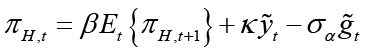
κ is defined as the identity κ ≡ λ(σα + φ) and λ is defined as 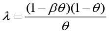 . φ represents inverse elasticity of labor supply and θ represents domestic price stickiness degree.14 κ depends on elasticity of labor supply and domestic price stickiness degree. Thus it is possible to interpret changes in κ as changes in inverse elasticity of labor supply and domestic price stickiness degree. Most studies examine changes in κ with relation to domestic price stickiness degree. In this context, Kuttner and Robinson (2010) argue that the reason for the change in the slope of the New Keynesian Phillips curve is basically a change in price-setting behavior. Rogoff (2003) and Rogoff (2006) explain the effects that cause the change in price-setting behavior in two different ways. The first is that globalization increases price elasticities (i.e., θ decreases). The second is that increasing competition reduces the mark-ups of goods and services. Rogoff (2003) and Rogoff (2006) argue that both these effects will increase the slope of the New Keynesian Phillips curve. Therefore, he claims that policymakers are faced with a short-term output-inflation equilibrium as the slope of the New Keynesian Phillips curve increases. The slope of the New Keynesian Phillips curve is
  and its parameter is κ. Thus, the lower marginal cost elasticity15 in relation to the real level of economic activity leads to a lower κ (steeper slope). This situation can be interpreted as the convergence of the New Keynesian Phillips curve from short run to long run.
Social loss is calculated using unconditional variance as in the studies by Woodford (2003) and Saulo et al. (2013). In order to calculate the expected loss of the objective (loss) function of the monetary and fiscal policymaker, these loss functions are defined with a description similar to the process in the following figure;


In the light of the calibrated parameters in Table 1, the variance and social loss values for different κ values of each policymaker are shown in Table 6.
The values in Table 6 show the social loss function values obtained as a result of game theoretical analysis of alternative scenarios of interaction between policymakers. κ value of the model calibrated with data from Turkey was found to be 1.5. This is the scenario with less social loss where the monetary policymaker is the leader and 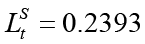 . In addition, in the scenario where the monetary policymaker is the leader in all alternative κ values, social loss is always lower. This result shows that in terms of social loss the policy coordination where fiscal policymaker is the leader is more unsuccessful for Turkey. It has been mentioned that the alternative κ values theoretically give us some inferences about the New Keynesian Phillips curve. In order to examine which scenario yields better results with alternative κ values, namely the increase or decrease of price elasticities (short-term and long-term distinction), we can use the behavior of monetary, fiscal and social loss functions depending on the alternative κ values in Table 6 or more clearly in Figure 2.
Table 6. Social Loss Values of Alternative Scenarios
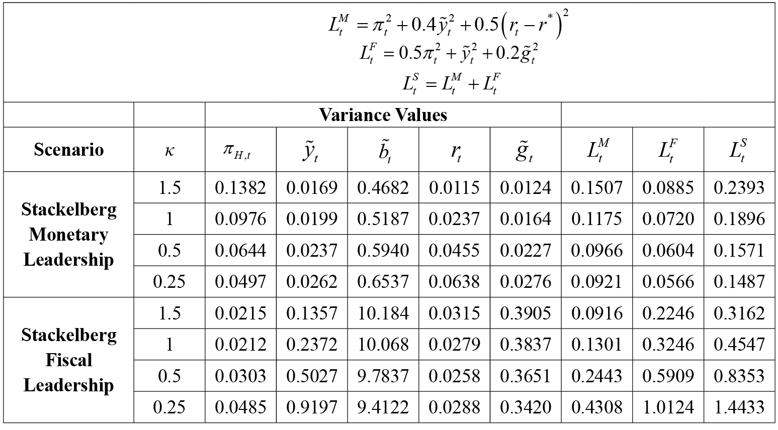
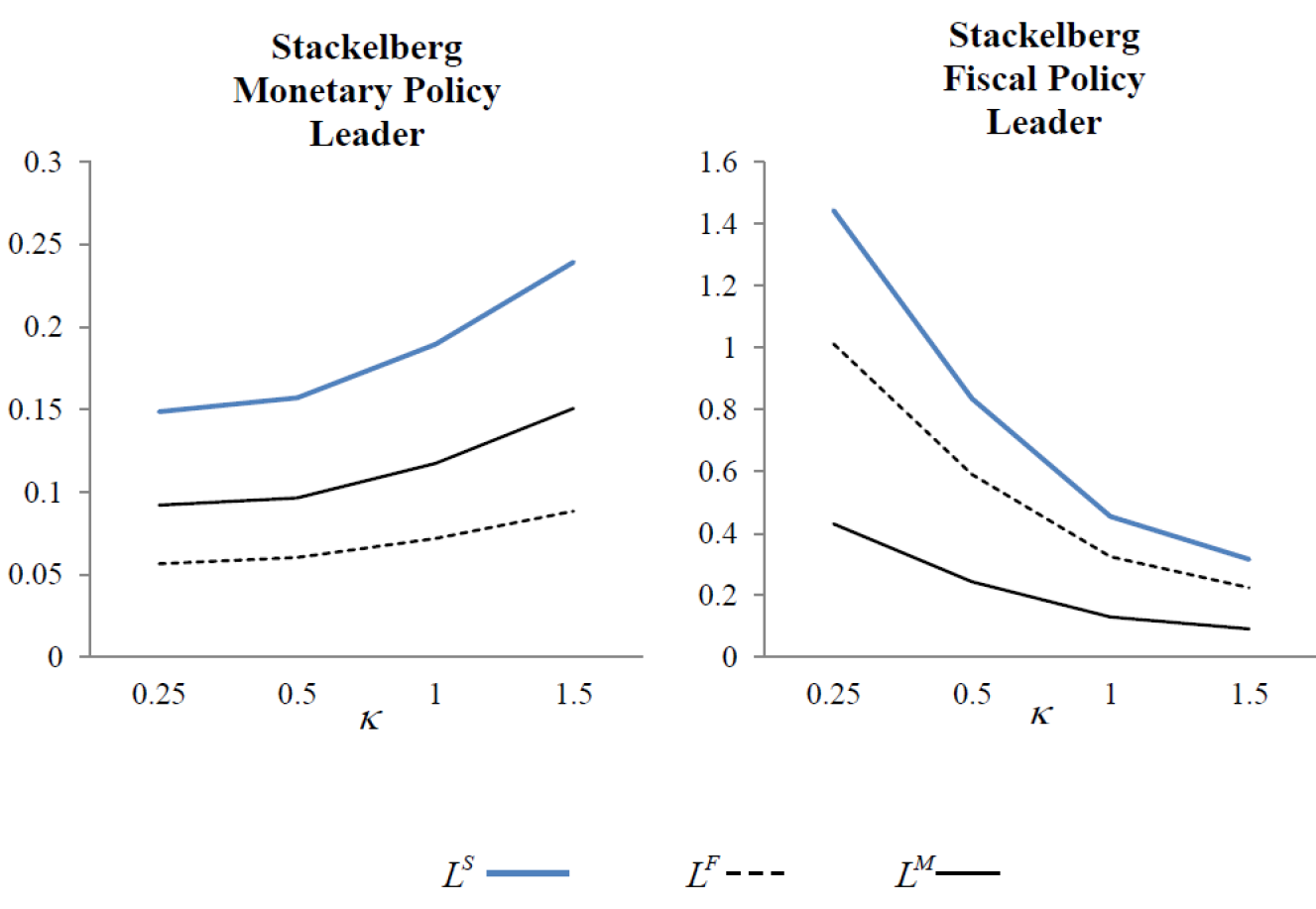
Figure 2. Behavior of Monetary, Fiscal and Social Loss Values Depending on Alternative κ Values
The results for the periodic changes in social loss values are presented in Figure 2. Looking at Figure 2, it is seen that social loss values change as alternative κ values change. For example, as the alternative κ values decrease (i.e., as they approach long-term conditions), the social loss value decreases in the scenario where monetary policymaker is the Stackelberg leader and decreases in the other scenario. On the contrary, as the alternative κ values increase (i.e., closer to short-term conditions), the social loss value increases in the scenario where monetary policymaker is the Stackelberg leader and decreases in the other scenario. In this framework, for the smallest value of κ (0.25), lowest social loss occurs when the monetary policymaker is the Stackelberg leader. Together with the information obtained from the studies of Rogoff (2006) and Ball (2006), policies to be followed by policymakers within the framework of short / long term output-inflation equilibrium according to the slope of the New Keynesian Phillips curve can be interpreted again with the findings obtained from Table 6 and Figure 2. Assuming that the New Keynesian Phillips curve has a high slope (low price elasticity / short-term), the best result in terms of social loss is reached with strategic interaction where the monetary policymaker is the Stackelberg leader and the fiscal policymaker is the follower. Moreover, for the case where the slope of the New Keynesian Phillips curve is low (high price elasticity / long term), it can be said that the scenario where the monetary policymaker is the leader will still give a better outcome for social loss.
5. Conclusion
Policymakers in many countries often emphasize the importance of coordination in ensuring macroeconomic stability in their reports. The problem here, however, is what kind of policy mix will provide coordination between policymakers in practice and the face of economic shocks. This study suggests a policy to ensure coordination between monetary policymaker that fights inflation and the fiscal policymaker which may or may not aid this objective. This policy proposal is based on the nature of the strategic interaction between policymakers. We do this by examining the interaction between monetary and fiscal policymakers within the framework of game theory, based on the New Keynesian macroeconomic model. The dynamic simulation method was used to evaluate the models derived from the game theoretically developed scenarios. In this method, some parameters in the model were calibrated using the information from previous studies and some other parameters were calibrated according to our calculations for the Turkish economy. Computational parameters were calibrated based on data from the Turkish economy in the period 2006: 01-2019: 12. Findings are sensitive to initial calibration as in the study by Van Aerle et al. (2002) et al. Different parameter values change the results of impulse-response and social loss analysis with the simulation of the models. This situation shows us that each general equilibrium model developed with optimal fiscal and monetary policies derived from game theory will yield different findings for other countries’ economies. It can also be said that incorrect parameter calibration can lead to false findings.
In the general equilibrium model developed on the structure of the strategic interaction between monetary and fiscal policymakers, when the responses of variables to an exogenous technology shock are examined, it is observed that monetary and fiscal policymakers both apply an expansionary policy mix whether or not they are the Stackelberg leader. When the responses of variables to an exogenous domestic price (negative supply) shock are analyzed, in both scenarios, the monetary policymaker gives a contractive policy response, while the fiscal policymaker gives an expansionary policy response. The responses of these policy mixes are similar to those in Çebi (2012) and Fragetta and Kirsanova, (2010) who also investigated the optimal interaction. The impact of this shock disappears in similar periods in both scenarios. However, when the dynamic nature of a negative supply shock is analyzed by comparing response sizes, it is thought that the worse policy mix is the scenario where the fiscal policymaker is the leader.
An important finding is encountered in terms of strategic interaction between policymakers when the effect of a positive nominal interest rate shock (a contractionary monetary policy shock) and a positive government spending shock (expansionary fiscal policy shock) is assessed. The fiscal policymakers give a contractionary response to the contractionary policy move of the monetary policymaker when the fiscal policymaker is the Stackelberg leader, yet it gives an expansionary response when the monetary policymaker is the Stackelberg leader. This is because the fiscal policymaker responds after the move of its follower i.e., with a lag when it is the leader. With the effect of the lag, high-interest rates caused by the follower monetary policymaker lead to high debt accumulation. Also, in the impulse response analysis of the scenario where the fiscal policymaker is the Stackelberg leader, it is seen that the debt stock responds positively to an increase in interest rate. In this framework, it appears that the fiscal policymaker applies a contractionary policy by reducing government spendings to stabilize the debt stock. The monetary policymakers give a contractionary response to the expansionary policy move of the fiscal policymaker when the fiscal policymaker is the Stackelberg leader. However, this response occurs with a lag when the monetary policymaker is the Stackelberg leader. The fact that the leading monetary policymaker determines its policy rule independent of the move of its follower (expansionary fiscal policy) and responses with a lag shows that this is a period of high inflation and debt stock. The only scenario where inflation and debt stock respond positively appears to be the case where monetary policymaker is the Stackelberg leader.
As a result of the impact-response analysis, when the dynamic nature of shocks is examined, it is seen that the best policy mix performance in terms of social loss the scenario where the monetary policymaker is the Stackelberg leader. However, this finding needs strengthening. In this context, it is investigated what policy mix is best for the Turkish economy in terms of social losses. In this analysis, the slope of the Phillips curve, which has an impact on the effectiveness of the contractionary and expansionary policies implemented by policymakers, should also be taken into consideration. As a result of the game-theoretical examination of the interaction between policymakers, it is concluded that the scenario that minimizes social loss for the Turkish economy is when the monetary policymaker is the Stackelberg leader. In addition, this conclusion is observed to be true both when the slope of the Phillips curve is high (i.e., it approaches short-term conditions) and when it decreases (i.e., it approaches long-term conditions).
In subsequent studies, small open dynamic stochastic equilibrium models developed with game theoretically derived optimal fiscal and monetary policies can be estimated for Turkey and/or other countries. Predictions made for Turkey can be separated for periods when policymakers interact with or without cooperation. Game theoretically derived optimal fiscal and monetary policies in this study allow this.
References
Ball, L. M. (2006). Has globalization changed inflation? (No. w12687). National Bureau of Economic Research.
Bilgin, B. A. R. İ., & Şıklar, İ. (2016). Enflasyon Hedeflemesi Rejiminde Para Politikasının Analizi: Türkiye İçin Dinamik Stokastik Genel Denge Modeli Tahmini. Anadolu Üniversitesi Sosyal Bilimler Dergisi, Vol. 16, issue 5, p. 47-70. https://doi.org/10.18037/ausbd.417429
Blinder, A. S. (1983). Issues in the coordination of monetary and fiscal policy.
Buti, M., Roeger, W., & Veld, J. I. T. (2001). Stabilizing Output and Inflation: Policy Conflicts and Co-operation under a Stability Pact. JCMS: Journal of Common Market Studies, Vol. 39, issue 5, p. 801-828. https://doi.org/10.1111/1468-5965.00332
Çebi, C. (2012). The interaction between monetary and fiscal policies in Turkey: An estimated New Keynesian DSGE model. Economic Modelling, Vol. 29, issue 4, p.1258-1267. https://doi.org/10.1016/j.econmod.2012.04.014
Di Bartolomeo, G., & Di Gioacchino, D. (2004). Fiscal-monetary policy coordination and debt management: a two stage dynamic analysis. University of Roma “La Sapienza”, mimeo.
Flotho, S. (2012). Monetary and fiscal policy in monetary union under the zero lower bound constraint (No. 20). Discussion Paper Series, University of Freiburg, Department of International Economic Policy.
Fragetta, M., & Kirsanova, T. (2010). Strategic monetary and fiscal policy interactions: An empirical investigation. European Economic Review, Vol. 54, issue 7, p. 855-879. https://doi.org/10.1016/j.euroecorev.2010.02.003
Gali, J., & Monacelli, T. (2005). Optimal monetary and fiscal policy in a currency union (No. w11815). National Bureau of Economic Research.
Gali, J., & Monacelli, T. (2008). Optimal monetary and fiscal policy in a currency union. Journal of international economics, Vol. 76, issue 1, p. 116-132. https://doi.org/10.1016/j.jinteco.2008.02.007
Galí, J. (2015). Monetary policy, inflation, and the business cycle: an introduction to the new Keynesian framework and its applications. Princeton University Press.
Giannoni, M. P., & Woodford, M. (2002a). NBER working paper series: Vol. 9419. Optimal interest-rate rules: I. General theory.
Giannoni, M. P., & Woodford, M. (2002b). NBER working paper series: Vol. 9420. Optimal interest-rate rules: II. Applications.
Henry, B., Nixon, J., & Hall, S. (1999). Central Bank Independence and Co-ordinating Monetary and Fiscal Policy. Economic Outlook, Vol. 23, issue 2, p. 7-13.
IMF and World Bank, 2003. Guidelines for Public Debt Management. Washington, D.C.:IMF.
Kirsanova, T., Stehn, S. J., & Vines, D. (2005). The interactions between fiscal policy and monetary policy. Oxford Review of Economic Policy, Vol. 21, issue 4, p. 532-564.
Kuttner, K., & Robinson, T. (2010). Understanding the flattening Phillips curve. The North American Journal of Economics and Finance, Vol. 21, issue 2, p. 110-125. https://doi.org/10.1016/j.najef.2008.10.003
Lambertini, L., & Rovelli, R. (2003). Monetary and fiscal policy coordination and macroeconomic stabilization. A theoretical analysis.
Lubik, T. A., & Schorfheide, F. (2007). Do central banks respond to exchange rate movements? A structural investigation. Journal of Monetary Economics, Vol. 54, issue 4, p. 1069-1087. https://doi.org/10.1016/j.jmoneco.2006.01.009
Neck, R. (1999). Dynamic games of fiscal and monetary policies for Austria. Annals of Operations Research, Vol. 88, p. 233-249.
Nordhaus, W. D. (1994). Policy Games: Coordination and Independence in Monetary and Fiscal Policies”, Brookings Papers on Economic Activity, Vol. 2, p. 139-216.
Raspudić, G., Z. (2012). Coordination between the monetary and public debt management policies in Croatia. Financial Theory and Practice, Vol. 36, issue 2, p. 109-138.
Rogoff, K. (2003). Globalization and global disinflation. Economic Review-Federal Reserve Bank of Kansas City, Vol. 88, issue 4, p. 45.
Rogoff, K. (2006, August). Impact of globalization on monetary policy. In a symposium sponsored by the Federal Reserve Bank of Kansas City on “The new economic geography: effects and policy implications”, Jackson Hole, Wyoming (pp. 24-26).
Sargent, T. J., & Wallace, N. (1981). Some unpleasant monetarist arithmetic. In Monetarism in the United Kingdom (pp. 15-41). Palgrave Macmillan UK.
Saulo, H., Rêgo, L. C., & Divino, J. A. (2013). Fiscal and monetary policy interactions: a game theory approach. Annals of Operations Research, Vol. 206, issue 1, p. 341-366.
Snowdon, B., & Vane, H. (1995). New-Keynesian economics today: the empire strikes back. The American Economist, Vol. 39, issue 1, p. 48-65. https://doi.org/10.1177%2F056943459503900107
Telatar, Erdinç, Funda Erdoğan. (1997). Para Politikası Oyununda İnandırıcılık, Ankara: Hacettepe Üniv. İ.İ.B.F. Yayınları, No:25.
Tetik, M., & Ceylan, R. (2016). Investigation of Interaction Between Monetary and Fiscal Policy in Turkey: SVAR Approach. Journal of Multidisciplinary Developments, Vol. 1, issue 1, p. 113-121.
Tetik, M., & Ceylan, R. (2017). Prisoner dilemma between policy makers: Evidence from Turkey. Bizinfo (Blace), Vol. 8, issue 2, p. 1-13.
Van Aarle, B., Bovenberg, L., & Raith, M. (1995). Monetary and fiscal policy interaction and government debt stabilization. Journal of Economics, Vol. 62, issue 2, p. 111-140. https://doi.org/10.1007/BF01226006
Van Aarle, B., Di Bartolomeo, G., Engwerda, J., & Plasmans, J. (2002). Monetary and fiscal policy design in the EMU: an overview. Open economies review, Vol. 13, issue 4, p. 321-340. https://doi.org/10.1023/A:1020609312575
Woodford, M. (2003). Interest and prices: foundations of a theory of monetary policy. Princeton: Princeton University Press.
Appendix-1: The Optimal Interest Rate Rule in the Framework of the Non-cooperative Nash Game
The monetary policymaker aims to minimize the loss function 4, which corresponds to the equilibrium condition of the economy. Thus, the monetary policymaker will act according to the optimal policy rule when the moves are made simultaneously. In the loss function; γπ, γy and γr are positive weights on the square of the deviation of current inflation from the inflation target, the square of the output gap and the square of the deviation of the interest rate from the equilibrium interest rate, respectively. The aim of the monetary policymaker is to solve the following problem, considering the constraints in the economy.
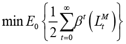
The following equations 1 and 2, which was previously defined, are constraint equations:

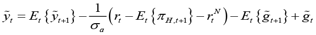
We obtain the optimal interest rate rule (NCN: Non-Cooperative Nash) by writing these problems as the Lagrange equations as in Woodford (2003) and then solving their first order conditions. The Lagrange structure of this problem is as follows:
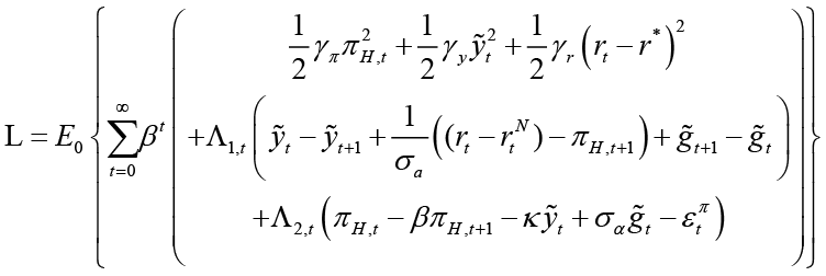
To write first-order conditions, the derivative this equation with respect to (rt – r*) and state variables (πH,t and  ) must be taken. Before moving forward, we must consider how we are going to handle terms of expectation in constraint. Since this is a policy under commitment, removing the expectation operator catches the idea of policymakers choosing an old rule to follow in the future. Hence, the inflation, output gap and government spending expectation operator at t + 1 have been removed. For example, if the inflation rate determined by the policymaker affects both current and expected inflation, then the policy authority can directly optimize both (Saulo et al., 2013).
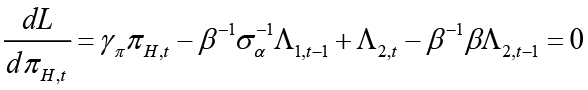
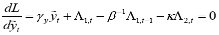
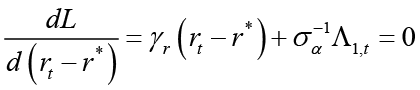
From Lagrange multipliers we find: 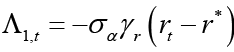 and
and  . As a result of the required replacement and separation process, the optimal nominal interest rule is obtained as follows17;
 (8)
(8)
In equation 8,  ,
,  ,
,  ,
, 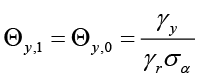 and
and 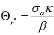 , respectively.
Appendix-2: The Optimal Spending Rule in the Framework
of the Non-Cooperative Nash Game
The fiscal policymaker aims at minimizing the loss function 5, which corresponds to the equilibrium condition of the economy. 18 Thus, the monetary policymaker will act according to the optimal policy rule when the moves are made simultaneously. In the loss function; ρπ, ρy and ρg are positive weights on the square of the deviation of current inflation from the inflation target, the square of the output gap and the square of the deviation of the interest rate from the equilibrium interest rate, respectively. The aim of the fiscal policymaker is to solve the following problem, considering the constraints in the economy.
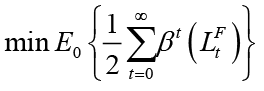
The following equations 1 2, and 3, which was previously defined, are constraint equations:
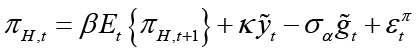

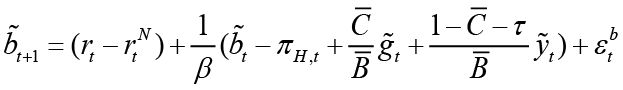
Again, we obtain the optimal interest rate rule  by writing these problems as the Lagrange equations and then solving their first order conditions. Thus, the non-cooperative optimal nominal spending rule is obtained as;19

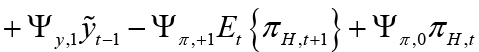 (9)
(9)
In equation 9, 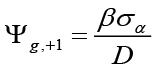 ,
, 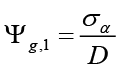 ,
, 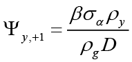 ,
, 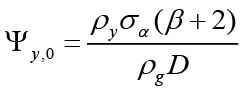 ,
,  ,
, 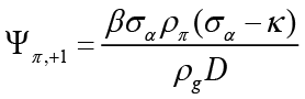 ,
, 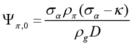 and finally
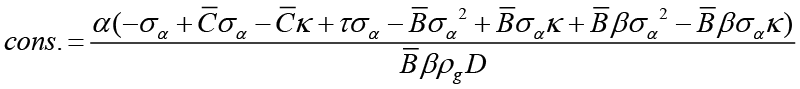 ’dir. Also, we define
 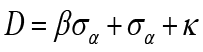 for the sake of simplicity.
Equation 9 is the rule that the fiscal policymaker commits to follow, and this rule can be called the non-cooperative Nash spending rule. The non-cooperative Nash spending rule has been linked to expected and current inflation, expected, current and past output gap, and finally past and expected government spending. The spending rule includes forward and backward dependence as it reacts to past and future government spending.
1 In explicit form, 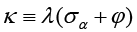 where
where 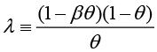 and
and 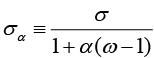 . In these equations, φ represents the supply elasticity of workforce, β represents the inter-period discount rate which defines the time preference rates, θ represents price rigidity degree, σ represents inter-period substitution flexibility and α represents the openness index. In explicit form,
 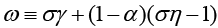 . In this equation the γ represents the substitution flexibility between goods produced in different foreign countries and η represents the substitution elasticity between domestic and foreign goods.
2 In the equation for natural interest rate, ρa represents the AR coefficient of natural productivity level and  represents AR coefficient of World output.
3 Since the natural level of inflation  is assumed
  , πt is used in the budget deficit equation.
4 Giannoni and Woodford (2003) define the optimal policy rule derived with this approach as “Robust Optimal Policy Rule”. This policy rules do not depend on the characteristics of exogenous shocks in the model. Thereby Giannoni and Woodford (2003) emphasize that the derived optimal policy rules are “robust” against misspecification.
5 Since the natural level of inflation is assumed  ,
,  is used in the fundamental equations instead of
  and
and  .
.
6 In the flexible price economy, government spending and taxes are assumed to be zero, which means there is no budget deficit or surplus under the flexible price equilibrium. Thus, it is safe to say .
.
7 Derivation of the optimal spending rule in the framework of the non-cooperative Nash game can be seen in Appendix 1.
8 It has been tried to obtain the optimal interest rate rule ( ) by writing these problems as Lagrange equation as in Woodford (2003) and then solving their first order conditions. However, since the obtained equation system did not have an analytical solution, the unconstrained optimization technique was used. The optimal policy rule derived by this technique cannot be expressed as “Robustly Optimal Policy Rule” because the derived policy rules depend on the characteristics of the exogenous shocks in the model.
9 Appendix Table 1 provides the solution of the optimal interest rate rule with Maple 11 when monetary policy maker is the Stackelberg leader. Appendix Table 3 has been uploaded to the journal system as a research material; it can be obtained here
10 Derivation of the optimal interest rate rule in the framework of the non-cooperative Nash game can see in Appendix 1.
11 It has been tried to obtain the optimal interest rate rule ( ) by writing these problems as Lagrange equation as in Woodford (2003) and then solving their first order conditions. Again, since the obtained equation system did not have an analytical solution, unconstrained optimization technique was used. The optimal policy rule derived by this technique cannot be expressed as “Robustly Optimal Policy Rule”as stated in footnote no.11.
12 Appendix Table 2 provides the solution of the optimal spending rule with Maple 11 when fiscal policy maker is the Stackelberg leader. Appendix Table-4 has been uploaded to the journal system as a research material. it can be obtained here
13 Gali and Monacelli (2008) explained the source of the negative relationship between marginal cost and government spending in their study. At a given level of output, an increase in government spending increases domestic consumption and / or creates real appreciation. These two situations tend to have a negative impact on the product price (expected labor cost) and the real marginal cost.
14 Here, θ represents the invariance of prices, the measure (1 – θ) determines the prices of firms. The expected time between firms’ price adjustments is  .
.
15 The New Keynesian Philips Curve Equation becomes 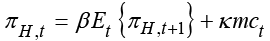 given that marginal costs are
 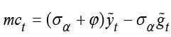 .
.
16 The constant 1/2 in this problem is just the scaling term that does not affect the optimality but somewhat simplifies the solution of the optimization problem..
17 Appendix Table 3 provides the solution of the optimal interest rate rule with Maple 11 in the framework of the non-cooperative Nash game. Appendix Table-1 has been uploaded to the journal system as a research material. it can be obtained here.
18 This loss function is similar to the one in the paper by Kirsanova et al. (2005).
19 Appendix Table 4 provides the solution of the optimal spending rule with Maple 11 in the framework of the non-cooperative Nash game. Appendix Table-2 has been uploaded to the journal system as a research material. it can be obtained here