Ekonomika ISSN 1392-1258 eISSN 2424-6166

2021, vol. 100(2), pp. 63–83 DOI: https://doi.org/10.15388/Ekon.2021.100.2.3

Fiscal Policy as a Solution to Involuntary Unemployment

Yasuhito Tanaka
Faculty of Economics, Doshisha University, Japan
Email: yatanaka@mail.doshisha.ac.jp

Abstract. We show the existence of involuntary unemployment based on consumers’ utility maximization and firms’ profit maximization behavior under monopolistic competition with increasing, decreasing or constant returns to scale technology using a three-periods overlapping generations (OLG) model with a childhood period as well as younger and older periods, and pay-as-you-go pension for the older generation, and we analyze the effects of fiscal policy financed by tax and budget deficit (or seigniorage) to achieve full-employment under a situation with involuntary unemployment. Under constant prices we show the following results. 1) If the realization of full employment will increase consumers’ disposable income, in order to achieve full-employment from a state with involuntary unemployment, we need budget deficit (Proposition 1). 2) If the full-employment state has been achieved, we need balanced budget to maintain full-employment (Proposition 2). We also consider fiscal policy under inflation or deflation. Additionally, we present a game-theoretic interpretation of involuntary unemployment and full-employment. We also argue that if full employment should be achieved in equilibrium, the instability of equilibrium can be considered to be the cause of involuntary unemployment.
Key Words: Involuntary unemployment, Three-periods overlapping generations model, Monopolistic competition, Nash equilibrium.

_________

Received: 08/04/2021. Revised: 22/05/2021. Accepted: 25/05/2021
Copyright © 2021 Yasuhito Tanaka. Published by Vilnius University Press
This is an Open Access article distributed under the terms of the Creative Commons Attribution License, which permits unrestricted use, distribution, and reproduction in any medium, provided the original author and source are credited.

1. Introduction

In this paper we analyze the effects of fiscal policy to achieve full-employment under a situation with involuntary unemployment. Involuntary unemployment in this paper is a phenomenon that workers are willing to work at the market wage or just below but are prevented by factors beyond their control, mainly, deficiency of aggregate demand. Umada (1997) derived an upward-sloping labor demand curve from the mark-up principle for firms, and argued that such an upward-sloping labor demand curve leads to the existence of involuntary unemployment without wage rigidity¹. But his model of firm behavior is ad-hoc. Otaki (2009) says that there exists involuntary unemployment for two reasons: (i) the nominal wage rate is set above the reservation nominal wage rate; and (ii) the employment level and economic welfare never improve by lowering the nominal wage rate. He assumes indivisibility (or inelasticity) of individual labor supply, and has shown the existence of involuntary unemployment using efficient wage bargaining according to McDonald and Solow (1981). The arguments of this paper, however, do not depend on bargaining. If labor supply is indivisible, it may be 1 or 0. On the other hand, if it is divisible, it takes a real value between 0 and 1. As discussed by Otaki (2015) (Theorem 2.3) and Otaki (2012), if the labor supply is divisible and very small, no unemployment exists². However, we show that even if labor supply is divisible, unless it is so small, there may exist involuntary unemployment. We consider consumers’ utility maximization and firms’ profit maximization in an overlapping generations (OLG) model under monopolistic competition according to Otaki (2007, 2009, 2011, 2015), and demonstrate the existence of involuntary unemployment without the assumption of wage rigidity.

Also we analyze the effects of fiscal policy financed by tax and budget deficit (or seigniorage). Under constant prices we show the following results.

1. If realization of full employment will increase consumers’ disposable income, in order to achieve full-employment from a state with involuntary unemployment, we need budget deficit. (Proposition 1)

2. If the full-employment state has been achieved, we need balanced budget to maintain full-employment. (Proposition 2)

From these results we can say that additional government expenditure to achieve full-employment should be financed by seigniorage not public debt. We also analyze fiscal policy under inflation or deflation.

In the next section we analyze and show the existence of involuntary unemployment under monopolistic competition with increasing or decreasing or constant returns to scale technology using a three-periods OLG model with a childhood period as well as younger (working) and older (retired) periods. Also we consider a pay-as-you-go pension system for the older generation. The simple two-periods OLG model falls in the nominal wage rate, and the prices of goods may increase consumption and employment by the so-called real balance effect. In such a model, consumers have savings for future consumption, but no debt. In a three-periods model with the childhood period, they consume goods in their childhood period by borrowing money from (employed) consumers of the previous generation and/or scholarships, and must repay their debts in the next period. The real value of the debt is increased by falls in the nominal wage rate and the prices. In addition to this configuration we consider a pay-as-you-go pension system for the older generation which may reduce the savings of consumers. Then, consumptions and employment may decrease by falling of the nominal wage rate. We think that our model is more general and realistic than a simple two-periods OLG model. In Section 3 we examine the effects of a fall in the nominal wage rate. In our three-periods OLG model with pay-as-you-go pension increases in consumption and employment due to falls in the nominal wage rate, and the prices of the goods might be negative. In that case, if full employment should be achieved in equilibrium, the instability of equilibrium can be considered to be the cause of involuntary unemployment.

In Section 4 we study the fiscal policy financed by tax and budget deficit (or seigniorage) to achieve full-employment at a state with involuntary unemployment. Additionally we present a game-theoretic interpretation of involuntary unemployment and full-employment in Section 5.

As we will state in the concluding remarks, the main limitation of this paper is that the goods are produced by only labor and there exists no capital and investment of firms. A study of the problem of involuntary unemployment and fiscal policy in such a situation is the theme of future research.

Schultz (1992) showed that there does not exist involuntary unemployment in the overlapping generations model. His argument depends on the real balance effect on consumption of the older generation’s consumers. We consider a three generations overlapping generations model with pay-as-you-go pension to explore the possibility of avoiding the real balance effect. See Section 3.

As we will show in Section 4.4, our discussion is closely related to the so-called functional finance theory by Lerner (1943, 1944) and Modern Monetary Theory (MMT, Mitchell, Wray and Watts (2019), Kelton (2020)).

2. Existence of involuntary unemployment

2.1. Consumers

We consider a three-periods (0: childhood, 1: younger or working, and 2: older or retired) OLG model under monopolistic competition. It is a re-arrangement and an extension of the model put forth by Otaki (2007), (2009), and (2015). The structure of our model is as follows.

1. There is one factor of production, labor, and there is a continuum of perishable goods indexed by z ∈ [0,1]. Good z is monopolistically produced by firm z with increasing or decreasing or constant returns to scale technology.

2. Consumers consume the goods during the childhood period (Period 0). This consumption is covered by borrowing money from (employed) consumers of the younger generation and/or scholarships. They must repay these debts in their Period 1. However, unemployed consumers cannot repay their own debts. Therefore, we assume that unemployed consumers receive unemployment benefits from the government, which are covered by taxes on employed consumers of the younger generation.

3. During Period 1, consumers supply l units of labor, repay the debts and save money for their consumption in Period 2. They also pay taxes for the pay-as-you-go pension system for the older generation.

4. During Period 2, consumers consume the goods by using their savings carried over from their Period 1 earnings, and receive the pay-as-you-go pension, which is a lump-sum payment. It is covered by taxes on employed consumers of the younger generation.

5. Consumers determine their consumptions in Periods 1 and 2 and the labor supply at the beginning of Period 1. We assume that their consumption during the childhood period is constant.

Further we make the following assumptions

Ownership of firms: Each consumer inherits ownership of the firms from the previous generation. Corporate profits are distributed equally to consumers.

Zero interest rate: We assume zero interest rate, and that repayment of the debts of consumers in their childhood period is assured. Consumer borrowing in childhood period is constant. If the savings of consumers in the younger period are insufficient for the borrowing, the government lends the scholarship to consumers in the childhood period. Consumers in the younger period are indifferent between lending money to childhood period consumers and savings by money.

Due to the existence of pay-as-you-go pension, the savings may be insufficient to borrowing when consumption by consumers in the childhood period is not so small.

Notation

We use the following notation.

C_i^e : consumption basket of an employed consumer in Period i, i = 1.2.

C_i^u : consumption basket of an unemployed consumer in Period i, i = 1.2.

c_i^e (z): consumption of good z of an employed consumer in Period i, i = 1.2.

c_i^u (z): consumption of good z of an unemployed consumer in Period i, i = 1.2.

D: consumption basket of an individual in the childhood period, which is constant.

P_i: the price of consumption basket in Period i, i = 1,2.

p_i(z): the price of good z in Period i, i = 1,2.

: (expected) inflation rate (plus one).

W: nominal wage rate.

R: unemployment benefit for an unemployed individual. R = D.

: consumption basket in the childhood period of a next generation consumer.

Q: pay-as-you-go pension for an individual of the older generation.

Θ: tax payment by an employed individual for the unemployment benefit.

: pay-as-you-go pension for an individual of the younger generation when he retires.

Ψ: tax payment by an employed individual for the pay-as-you-go pension.

Π: profits of firms which are equally distributed to each consumer.

l: labor supply of an individual.

Γ(l): disutility function of labor, which is increasing and convex.

L: total employment.

L_f: population of labor or employment in the full-employment state.

y(Ll): labor productivity, which is increasing or decreasing or constant with respect to ‘employment × labor supply’ (Ll).

We assume that the population L_f is constant. We also assume that the nominal wage rate is constant in this section. We examine the effects of a change in the nominal wage rate in Section 3.

We consider a two-step method to solve utility maximization of consumers such that:

1. Employed and unemployed consumers maximize their consumption baskets given the expenditure in each period.

2. Then, they maximize their utility by determining consumption baskets in Periods 1 and 2 given their income over two periods:

We define the elasticity of the labor productivity with respect to “employment × labor supply” as follows:

We assume that 1< ζ < 1, and ζ is constant. Increasing (decreasing or constant) returns to scale means ζ > 0 (ζ < 0 or ζ = 0).

Since the taxes for unemployed consumers’ debts are paid by employed consumers of the same generation, D and Θ satisfy the following relationship.

D(L_f – L)=LΘ.

This means

L(D + Θ) = L_f D.

The price of the consumption basket in Period 0 is assumed to be 1. Thus, D is the real value of the consumption in the childhood period of consumers.

Also, since the taxes for the pay-as-you-go pension system are paid by employed consumers of the younger generation, Q and Ψ satisfy the following relationship:

LΨ=L_f Q.

The utility function of employed consumers of one generation over three periods is written as

u(C₁^e , C₂^e , D) – Γ(l).

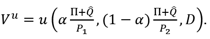
We assume that u(⋅) is a homothetic utility function. The utility function of unemployed consumers is

u(C₁^u , C₂^u , D).

The consumption baskets of employed and unemployed consumers in Period i are

and

σ is the elasticity of substitution among the goods, and σ > 1.

The price of consumption basket in Period i is

The budget constraint for an employed consumer is³

First, we consider the second step of utility maximization of consumers. The budget constraint for an unemployed consumer is

Since R = D,

Let

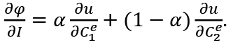
Since the utility functions u(C₁^e , C₂^e , D) and u(C₁^u , C₂^u , D) are homothetic, α is determined by the relative price , and does not depend on the income of the consumers. Therefore, we have

From the first order conditions and the budget constraints for employed and unemployed consumers we obtain the following demand functions for consumption baskets.

and

Lagrange functions in the first step for employed and unemployed consumers are

and

λ₁^e , λ₂^e, λ₁^u and λ₂^u are Lagrange multipliers. Upon solving these maximization problems, the following demand functions of employed and unemployed consumers are derived⁴.

and

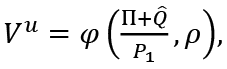
From these analyses we obtain the indirect utility functions of employed and unemployed consumers as follows:

and

Let

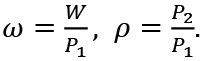
Then, since the real value of D in the childhood period is constant, we can write

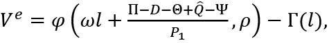
ω is the real wage rate. We denote

The condition for maximization of V^e with respect to l given ρ is

where

Given P₁ and ρ the labor supply is a function of ω. From (4) we get

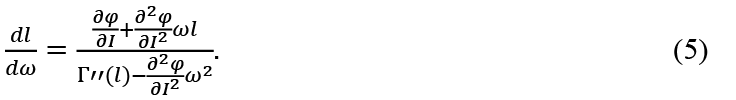
If , the labor supply is increasing with respect to the real wage rate ω.

2.2. Firms

Let d₁(z) be the total demand for good z by younger generation consumers in Period 1. Then:

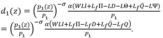
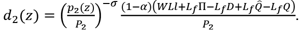
This is the sum of the demand of employed and unemployed consumers. We note that is the pay-as-you-go pension for younger generation consumers in their Period 2. Similarly, their total demand for good z in Period 2 is written as

Let be the demand for good z by the older generation. Then,

where and are the nominal wage rate, the profits of firms, the employment, the individual labor supply, the debt of an individual, and the pay-as-you-go pension, respectively, during the previous period. Q is the pay-as-you-go pension for consumers of the older generation themselves. Let

This is the total savings or the total consumption of the older generation consumers including the pay-as-you-go pensions they receive in their Period 2. It is the planned consumption that is determined in Period 1 of the older generation consumers. Net savings is the difference between M and the pay-as-you-go pensions in their Period 2, as follows:

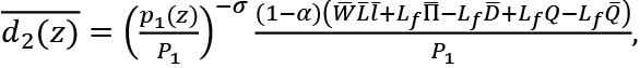
Their demand for good z is written as . Government expenditure constitutes the national income as well as the consumptions of the younger and older generations. Then, the total demand for good z is written as

where Y is the effective demand defined by

We note that is consumption in the childhood period of a next generation consumer. G is the government expenditure, except for the pay-as-you-go pensions, scholarships and unemployment benefits (see Otaki (2007), (2015) about this demand function). Now, we assume that G is financed by seigniorage similarly to Otaki (2007) and Otaki (2009). In a further section, we will consider the government’s budget constraint with respect to taxes.

Let L and Ll be employment and the ‘employment × labor supply’ of firm z. The total employment and the total ‘employment × labor supply’ are also

The output of firm z is Lly(Ll). At the equilibrium Lly(Ll) = d(z). Then, we have

From (6)

Thus

The profit of firm z is

The condition for profit maximization is

Therefore, we obtain

Let Then:

This means that the real wage rate is

With increasing (decreasing or constant) returns to scale,ω is increasing (decreasing or constant) with respect to “employment × labor supply” Ll.

From (3), (4) and (7), we have

with

Then, from (5)

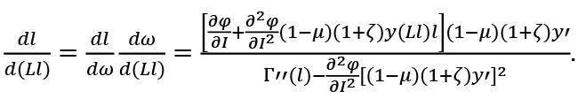
Assuming , with increasing (decreasing) returns to scale y' > 0 (y < 0), this is positive (negative). Since

and

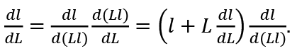
Thus:

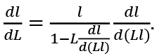
Usually and have the same sign, and we assume 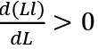in (8). Also, since -1 < ζ < 1, we have

Then, the output Lly(Ll) increases by an increase in L.

Since all firms are symmetric,

2.3. Involuntary unemployment

The (nominal) aggregate supply of the goods is equal to

The (nominal) aggregate demand is

Since they are equal,

or

In real terms⁵

or

From (4) and (5), the individual labor supply l is a (usually increasing) function of ω. From (7) ω is a function of Ll. With increasing (decreasing or constant) returns to scale technology, it is increasing (decreasing or constant) with respect to Ll or with respect to L given l. The individual labor supply l may be increasing or decreasing in L or Ll. However, we assume that Ll is increasing in L. This requires

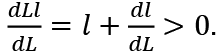
It means Ll < L_f l for L < L_f. The equilibrium value of Ll cannot be larger than L_f l. However, it may be strictly smaller than L_f l. Then, we have L < L_f and involuntary umemployment exists.

If the government collects a proportional tax at the rate t from the younger generation consumers, the aggregate demand is

2.4. Discussion summary

The real wage rate depends on the elasticity of the labor productivity with respect to ‘employment × labor supply’ and the employment level. But the employment level does not depend on the real wage rate. The real aggregate demand and the employment level are determined by the value of

If the employment is smaller than the labor population, then involuntary unemployment exists.

2.5. The case of full-employment

If Ll = L_f l, full-employment is achieved. Then, (11) is re-written as

Since L_f and L_f l are constant (if L =L_f, ω is constant), this is an identity not an equation. On the other hand, (11) is an equation not an identity. (13) should be written as

This yields:

Then, the nominal wage rate is determined by:

3. Effects of a fall in the nominal wage rate

In the model of this paper, no mechanism determines the nominal wage rate except at the full-employment state. For example, when the nominal value of G increases, the nominal aggregate demand and supply increase. If the nominal wage rate rises, the prices also rise. If, when G increases, the prices rise considerably, then the outputs might not increase, and involuntary unemployment might not decrease, either. If the prices do not rise or if they rise only slightly, involuntary unemployment decreases.

Let us examine the effects on employment of a fall in the nominal wage rate. A fall in the nominal wage rate induces falls in the prices of the goods (see (10)), and it does not directly rescue involuntary unemployment. Proposition 2.1 in Otaki (2016) says

Suppose that the nominal wage sags. Then, as far as its indirect effects on the aggregate demand are negligible, this only results in causing a proportionate fall in the price level. In other words, a fall in the nominal wage never rescues workers who are involuntarily unemployed.

However, indirect effects on aggregate demand due to a fall in the nominal wage rate may exist. We assume that falls in the nominal wage rate and the prices are not predicted by consumers. If the prices of the goods fall, the real value of the older generation’s savings increases. But, at the same time, falls in the prices of the goods increase the real value of the younger generation consumers’ debts.

The real values of the following variables will be maintained even when both the nominal wage rate and the prices fall.

G / P₁: the government expenditure.

/ P₁: consumption in the childhood period of a next generation consumer.

Q / P₁: pay-as-you-go pension for an older generation consumer.

/ P₁: pay-as-you-go pension for a younger generation consumer when he retires.

On the other hand, the nominal value of D and that of M – L_f Q, which is the older generation’s net savings, do not change. Therefore, from (12), whether a fall in the nominal wage rate increases or decreases the effective demand depends on whether

is positive or negative. This is the so-called real balance effect. If D and Q are large, (14) is negative, and a fall in the nominal wage rate increases involuntary unemployment⁶. In that case, if full employment should be achieved in equilibrium, the instability of equilibrium can be considered to be the cause of involuntary unemployment.

4. Analysis of fiscal policy

4.1. Steady state with constant employment under constant prices

First consider a steady state where the employment is constant. With constant employment the real wage rate and the labor supply do not change, thus the output also does not change. We assume also ρ = 1, that is, the constant prices of the goods. Consumers correctly predict that the prices are constant. Let t be the tax rate. Then,

At the steady sate it must be that and Thus,

The total savings of the younger generation including the pay-as-you-go pension are equal to M. Therefore,

This means

Thus, to maintain a state with constant employment and prices we need a balanced budget.

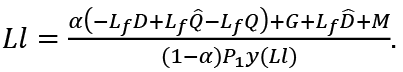
4.2. Fiscal policy for full-employment under constant prices

Next, let us consider a fiscal policy to achieve full-employment from the state with involuntary unemployment. The employment L and the output Lly(Ll) increase by fiscal policy. We assume constant prices of the goods again. Consumers correctly predict that the prices are constant. If the employment L increases, the labor supply l, the real wage rate ω and the labor productivity y(Ll) increase in the case of increasing returns to scale. However, in the case of decreasing returns to scale, the labor supply, the real wage rate and the labor productivity may decrease. In the former (latter) case the rate of increase in the output is probably larger (smaller) than the rate of increase in the employment. By (9) we can assume that both are positive.

Let G' and t' be the government expenditure and the tax rate to achieve full-employment. Then, (16) is written as

From this

Suppose , that is, the realization of full employment will increase the consumers’ disposable income. Then, from (17) and (19) we get

From this we obtain the following proposition.

Proposition 1 If the realization of full employment will increase consumers’ disposable income, in order to achieve full-employment from a state with involuntary unemployment, we need budget deficit.

Let G'', t'' and M' be the government expenditure, the tax rate and the total savings of the younger generation consumers in the next period after realization of full-employment. (16) is written as

To maintain full-employment, the total savings of the younger generation including the pay-as-you-go pension must be equal to M'. Then, we have

Therefore:

This means that in order to maintain full-employment, budget deficit is not required. Thus, we obtain the following proposition.

Proposition 2 If the full-employment state has been achieved by fiscal policy, we need a balanced budget to maintain full-employment.

A simple example

Let us assume M = 0 and T' = 0 in (18). Then:

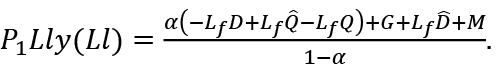
This means

This is the government expenditure necessary to achieve full employment, and it is equal to the total savings of the younger generation. Let us denote it by M'.

In the next period the following relation holds.

To maintain full-employment with t'' = 0 we need

Thus:

4.3. Realization of full-employment under inflation or deflation

First we assume that the output and the employment are constant, and the prices of the goods rise or fall at the rate ρ – 1. If ρ > 1(< 1), consumers correctly predict that the prices rise (fall). Let t be the tax rate. With ρ ≠ 0, and . Thus, (15) is written as

The total savings of the younger generation including the pay-as-you-go pension must be equal to ρM. Therefore,

This means that:

If M > L_f D + L_f Q, in order to maintain a state where the output and the employment are constant with rising prices (ρ > 1) (falling prices (ρ < 1)) a budget deficit (surplus) is required. If M < L_f D + L_f Q, we obtain the inverse results.

Let G' and t' be the government expenditure and the tax rate to achieve full-employment. Then, (20) is written as

From this

Suppose , that is, the realization of full employment will increase consumers’ disposable income. Then, from (21) and (23) we get

Therefore, in order to achieve full-employment under inflation (or deflation) we need budget deficit (or budget surplus) which is larger (smaller) than (22).

Let G'', t'', M' and P_1' be the government expenditure, the tax revenue, the total savings of the younger generation consumers and the price of the consumption basket in the next period after realization of full-employment. (20) is written as

To maintain full-employment, the total savings of the younger generation including the pay-as-you-go pension must be equal to ρM'. Then, we have

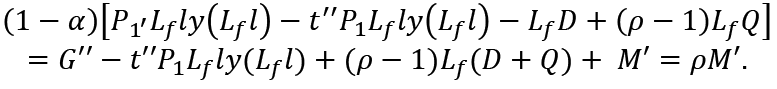
Therefore:

This means that in order to maintain full-employment, we need budget deficit (or surplus) which is equivalent to (22).

4.4. Relationship of our discussion to functional finance theory and MMT

The analysis of fiscal policy to achieve full employment in this paper is in line with the ideas of functional finance theory by, for example, Lerner (1943, 1944) and Forstater (1999), and this paper develops their arguments by using a simple mathematical model. In addition, the fact that this paper takes the position of the functional finance theory is similar to the Modern Monetary Theory (MMT, for example, Mitchell, Wray and Watts (2019), Kelton (2020)) that has recently attracted attention, and it can be said that this study is one of the attempts to present a mathematical model for the Modern Monetary Theory. A good or bad fiscal policy should be judged not by whether the fiscal balance is balanced or not, or whether the government debt will expand or not, but by whether full employment is achieved without causing high rates of inflation. Forstater says.

Policies should be judged on their ability to achieve the goals for which they are designed and not on any notion of whether they are ‘sound’ or otherwise comply with the dogmas of traditional economics (Forstater (1999)).

As shown in this paper, a budget deficit is necessary to achieve full employment from a state of involuntary unemployment, but once full employment has been achieved, it is maintained by a balanced budget, so it is not necessary to make up the budget deficit needed to get out of the recession with a budget surplus later.

In Japan, it is sometimes said that the fact that interest rates have remained low and prices have not risen in spite of a growing budget deficit is a phenomenon in line with MMT. However, Wray and Nersisyan (2021) say that this is not the case. The fact that Japan has a very large government debt, yet interest rates are low and prices have not risen defies the mainstream economics’ view of the dangers of government debt and budget deficits. However, Japan has not been successful in pulling itself out of the recession through fiscal policy. According to the empirical research by Wray and Nersisyan (2021), Japan has consistently chosen the path of stop-go fiscal measures. It has provided inadequate and temporary fiscal stimulus during recessions and then implemented austerity measures when the economy seemed to have recovered. They say ‘This has been justified on the basis of the following beliefs ‘Deficits and debt are too high’’.

5. Game-theoretic interpretation of involuntary unemployment and full-employment

A steady state under balanced budget with involuntary unemployment is in a Nash equilibrium of a game with firms and consumers.

1. Given the government expenditure and tax, and the strategies of consumers and other firms, each firm maximizes its profit. Consumers’ strategies are labor supply and consumption. Firms’ strategies are employment and production.

2. Given the government expenditure and tax, and the strategies of other consumers and firms, each employed consumer and each unemployed consumer maximize their utility. Each unemployed consumer determines his strategy given a state where he is not employed.

Further we present three more results.

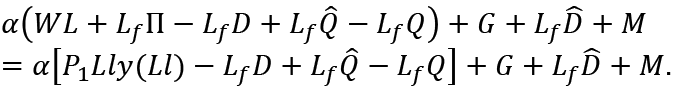
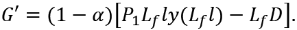
1. Increases in employment and production by firms and increases in labor supply and consumption by the younger generation consumers to the full-employment levels take the state out of the Nash equilibrium because consumption of the older generation consumers is insufficient. In this case, the aggregate supply is P₁L_f ly(L_f l), and the aggregate demand is

M and G are equal to M and G in (16) with G = tP₁L_f ly(L_f l). Then, the difference between P₁L_f ly(L_f l) and the left-hand side of (16) is

On the other hand, the difference between AD and the right-hand side of (16) is

Since 0 < α < 1, (25) is smaller than (24), and the aggregate demand is insufficient. The difference between (24) and (25) is

It is the deficiency of the savings of the older generation.

2. If the government increases its expenditure while keeping taxes intact, the full-employment state may be in a Nash equilibrium. The budget deficit makes up for deficiency of consumption of the older generation consumers.

3. Then, in the next period we can maintain full-employment without budget deficit because consumption of the older generation consumers, who work when they are young, is larger than the consumption of the older generation consumers in the previous period. This is a property of a dynamic OLG model.

6. Discussion and Concluding Remarks

From Propositions 1 and 2 we can say that in order to achieve full-employment from a state with involuntary unemployment, we need a budget deficit of the government. However, when full-employment is achieved, in order to maintain full-employment we need a balanced budget. Therefore, additional government expenditure to achieve full-employment should be financed by seigniorage not public debt.

We have examined the existence of involuntary umemployment and the effects of fiscal policy using a three-generation OLG model under monopolistic competition with increasing, decreasing or constant returns to scale. We considered the case of a divisible labor supply, and we assumed that the goods are produced only by labor.

In future research, we want to analyze involuntary unemployment and fiscal policy in a situation where goods are produced by capital and labor, and there exist investments of firms.

References

Forstater, M. (1999). Functional finance and full employment: Lessons from Lerner for today, Working Paper No. 272, Levy Economics Institute.

Hansen, G. D. (1985). Indivisible labor and the business cycle. Journal of Monetary Economics, 16(3), 309–327. https://doi.org/10.1016/0304-3932(85)90039-x

Kalecki, M. (1944). “The Classical Stationary State” A Comment. The Economic Journal, 54(213), 131. https://doi.org/10.2307/2959845

Kelton, S. (2020). The Deficit Myth: Modern Monetary Theory and the Birth of the People’s Economy. Public Affairs, Hatchette Book Group.

Lavoie, M. (2001). Efficiency Wages in Kaleckian Models of Employment. Journal of Post Keynesian Economics, 23(3), 449–464. https://doi.org/10.1080/01603477.2001.11490293

Lerner, A. P. (1943). Functional finance and the federal debt. Social Research, 10 (1), 38-51.

Lerner, A. P. (1944).The Economics of Control. New York: Macmillan.

McDonald, I. M., Solow, R. M. (1981). Wage bargaining and employment. American Economic Review, 71(5), 896–908.

Mitchell, W., Wray, L. R. and Watts, M. (2019). Macroeconomics. Red Gbole Press.

Otaki, M. (2007). The dynamically extended Keynesian cross and the welfare-improving fiscal policy. Economics Letters, 96(1), 23–29. https://doi.org/10.1016/j.econlet.2006.12.005

Otaki, M. (2009). A welfare economics foundation for the full-employment policy. Economics Letters, 102(1), 1–3. https://doi.org/10.1016/j.econlet.2008.08.003

Otaki, M. (2012). The aggregation problem in the employment theory: The representative individual model or individual employees model? Theoretical Economics Letters, 2(5), 530–533. 10.4236/tel.2012.25098

Otaki, M. (2015). Keynsian Economics and Price Theory: Re-orientation of a Theory of Monetary Economy. Springer.

Otaki, M. (2016). Keynes’s General Theory Reconsidered in the Context of the Japanese Economy. Springer.

Pigou, A. C. (1943). The classical stationary state. Economic Journal, 53(212), 343–351. https://doi.org/10.2307/2226394

Schultz, C. (1992). The impossibility of involuntary unemployment in an overlapping generations model with rational expectations. Journal of Economic Theory, 58(1)61–76. https://doi.org/10.1016/0022-0531(92)90101-M

Tanaka, Y. (2020a). Involuntary unemployment with indivisible labor supply under perfect competition. Economics Bulletin, 40(3),1914–1923.

Tanaka, Y. (2020b). Indivisible labor supply and involuntary unemployment: monopolistic competition model, The Singapore Economic Review, forthcoming.

Umada, T. (1997). On the existence of involuntary unemployment (hi-jihatsuteki-shitsugyo no sonzai ni tsuite (in Japanese)). Yamaguchi Keizaigaku Zasshi, 45(6), 61–73.

Wray, L. R., Nersisyan, Y. (2021). Has Japan Been Following Modern Money Theory

Without Recognizing It? No! And Yes, Working Paper No. 985, Levy Economics Institute.

Appendix

A. Some calculations

The first order condition for (2) is

From this

Then:

It means

and so

From (1)

Then:

Therefore:

Similarly:

Thus:

From (A.1)

By (A.1)

From this we get

and are similarly obtained.