Ekonomika ISSN 1392-1258 eISSN 2424-6166

2021, vol. 100(2), pp. 6–39 DOI: https://doi.org/10.15388/Ekon.2021.100.2.1

Risky Mortgages and Macroprudential Policy: A Calibrated DSGE Model for Lithuania

Jaunius Karmelavičius*
Financial Stability Department, Bank of Lithuania
Faculty of Economics and Business Administration, Vilnius University
Email: jkarmelavicius@lb.lt

Abstract. Following the financial crisis of 2009 there was an emergence of macroprudential policy tools, as well as a need to model the macroeconomy and the financial sector in a coherent framework. This paper develops and calibrates a small open economy DSGE model for Lithuania to shed some light on the interactions between the macroeconomy and the banking sector, regulated by macroprudential policy. The model features housing market, and endogenous credit risk a la de Walque et al. (2010), whereby the household can default on mortgage repayments, what leads to housing collateral seizure. Foreign-owned banks, that are subject to risk-sensitive macroprudential capital requirements, take into account not only the mortgage default rate but also the cap on loan to value (LTV) ratio when making lending decisions. Using this mechanism, we show that while a more stringent LTV constraint reduced credit demand, it can also lead to an expansion in credit supply via lower credit risk. Therefore, a tightening of LTV requirement should result in only a slight reduction in mortgage lending, coupled with lower interest rate margins. The article compares the impact of the tightening of three macroprudential tools, namely, bank capital requirements, mortgage risk weights and LTV limit. We find that broad-based capital requirements, such as the counter-cyclical capital buffer, are less efficient in leaning against the housing credit cycle, because of a relatively large cost incurred on the firm sector.
Keywords: macroprudential policy, mortgage defaults, LTV, capital requirements.

________

* The views expressed in this paper are those of the author and do not represent the official position of the Bank of Lithuania or the Eurosystem. Special thanks to Tomas Ramanauskas for his support, useful discussions and ideas. I would also like to thank discussant Oļegs Tkačevs for valuable comments at the 2nd Baltic Economic Conference (Riga, Latvia), as well as participants of seminars held at the Bank of Lithuania and Vilnius University, and central bank workshop Applications of DSGE Models in Central Banking (Kyiv, Ukraine), and conference Challenges of Europe: Growth, Competitiveness, Innovation and Well-being (Brač, Croatia). All errors are mine.

Received: 24/08/2021. Revised: 30/08/2021. Accepted: 02/09/2021
Copyright © 2021 Jaunius Karmelavičius. Published by Vilnius University Press
This is an Open Access article distributed under the terms of the Creative Commons Attribution License, which permits unrestricted use, distribution, and reproduction in any medium, provided the original author and source are credited.

1. Introduction

Over the recent decades loose monetary policy, financial deregulation and advances in finance greatly contributed to increasing financial leverage across the globe, thus fuelling asset prices in an unsustainable manner. This led to the biggest global financial crisis since the Great Depression. The past events revealed how banks, and the financial sector as a whole, are central to how the economy operates. Studies show (Claessens et al., 2009; Crowe et al., 2013; Jordà et al., 2013, 2017) that economic booms accompanied by rapid credit growth are usually associated with deeper and longer lasting recessions. Financial crises that are characterised by a credit crunch tend to be particularly severe.

The post-crisis period saw an emergence of macroprudential policy tools that address the systemic approach and are designed to decrease the formation of systemic risk and increase the resilience of markets, institutions and the general economy. This toolset is oriented towards banks and contains measures such as bank capital requirements and borrower-based measures, e.g. loan-to-value (LTV) ratio caps for mortgage lending, debt service to income (DSTI) and debt to income (DTI) ratio caps. In addition to improved regulation, the general failure to predict the financial crisis across the globe called for an extension of macroeconomic models to include financial frictions and housing.

This paper builds and calibrates a general equilibrium banking model for the economy of Lithuania, as the country experienced almost a textbook-type boom and bust cycle in the 2000’s, as well as had macroprudential regulation introduced in 2011, with measures such as DSTI cap of 40% and LTV cap 85% for mortgages, bank capital buffer requirements. The model features a small open economy with banking sector owned by a foreign household to reflect the structure of the banking sector in Lithuania.

From modelling standpoint, our contribution is that we use an alternative framework of endogenous mortgage defaults a la de Walque et al. (2010), coupled with multi-period loans as in Gelain et al. (2015, 2018) or Iacoviello (2015). Unlike other papers, e.g. Justiniano et al. (2015), we model defaults and bank asset seizure so that the LTV constraint is also a constraint on bank lending, not only on the borrower’s side. We keep a neat system of accounting identities for the firm and the banking sector, that relate to real-world accounting principles. Since the model is a stock-flow consistent system, with prices and banks that have nominal balance sheet identities, the banking sector is truly monetary in the sense that it features money creation as in Karmelavicius and Ramanauskas (2019).

We calibrate the model to match first moments of Lithuanian historical data and use it to simulate the short-term economic impact of macroprudential policy tools. Namely, we assess an increase in bank capital requirements and risk weights, as well as a tightening of mortgage LTV limits. A policy comparison exercise shows that broad-based capital requirements, such as the countercyclical capital buffer, are inferior to using more targeted measures like LTV cap and mortgage risk weights for reducing imbalances in the housing sector.

We proceed as follows: the next Section 2 describes the model we use for simulations, under the calibration from Section 3, Section 4 provides the analytical results and Section 5 concludes.

2. Model setup

This section describes the model which is a natural extension of Karmelavicius and Ra­manauskas (2019). The model features a small open economy setting without independent monetary policy¹. The figure below describes the sectors and agents of the economy and the financial flows among them. The macroeconomy is populated by two representative households, one of which is patient and the other one is impatient, as governed by lower discount factor. The motivation for this difference is that we want to introduce both household deposits and household debt into the model. Both households provide labour services to the firm sector and earn wages, whereas the patient also receives dividends as the owner of the firms. The patient household holds deposits in the banking sector that pay an interest rate, while the impatient can borrow and has to pay interest, and also has the ability to default on a fraction of the debt. Banks are foreign-owned and finance their activities by resorting to three resources of financing: deposits, foreign debt or bank capital. They extend loans to the corporate as well as the household sector. The corporate sector is populated by final good producers which operate in a perfectly competitive market, as well as intermediate producers which operate under monopolistic competition. The final good firms are essentially a packaging industry that buy intermediate goods as inputs. The intermediate firms accumulate physical capital and employ labour to produce a marginally distinctive variety. When referring to the firm sector, we usually refer to the intermediate firms, since final good producers are used only as a modelling device.

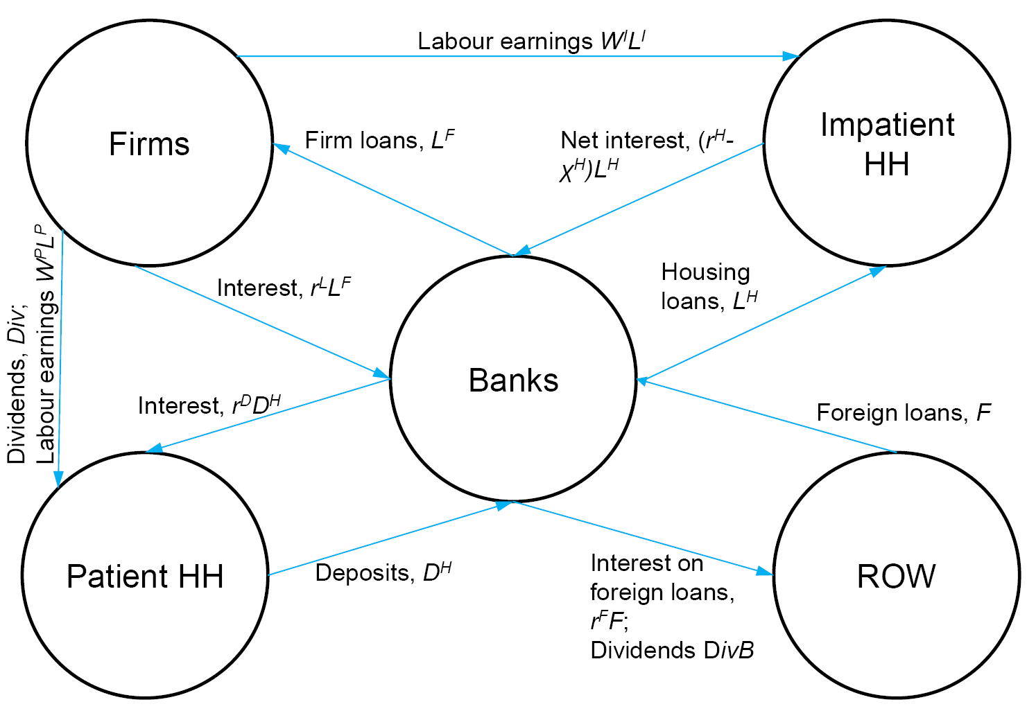
Figure 1. Schematic view of the financial flows within the model.

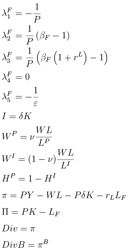
The model bears similarities to papers of Iacoviello (2005, 2015) and Gerali et al. (2010), de Walque et al. (2010), Vītola and Ajevskis (2011). In this setting we devote much attention to accounting identities (in nominal terms) of firms and banks for a realistic treatment. Most variables are nominal in the model, except consumption (C_t^s ), investment (I_t), output (Y_t), housing (H_t^s ), labour (L_t^s ), physical capital (K_t). In the remainder of this section we outline the model’s building blocks in more technical detail.

2.1. Households

The household sector is comprised of two representative households, one of which is patient and the other one is impatient. Since the patient household has a higher rate of time preference β_P > β_I, it is the depositor in this model, while the impatient one borrows from banks, subject to a collateral constraint. In addition, each provides labour services to the intermediate good sector, where their productivity is not necessarily identical. The patient household is assumed to be the owner of intermediate firms, thus receives dividends from them. Otherwise, both households are identical in their preferences, which are instituted in an identical instantaneous utility function:

where superscript ^P denotes the patient household and ^I the impatient. U_t^s is household’s utility at time t, C_t^s denotes consumption, H_t^s is housing and L_t^s is labour. σ_H and σ_L are weights in the utility function for housing and labour that are identical across households. We turn to describe each household in more detail.

2.1.1. Patient household

The patient household earns labour income, corporate dividends, interest on deposits and uses the proceeds to finance nominal consumption, accumulation of deposits and house purchases. The flow budget constraint is as follows:

where W_t^P is the patient’s nominal wage rate, Div_t denotes nominal dividends received from firms, D_t is the end of period t stock of nominal deposits and is the nominal interest rate on deposits held in period t – 1. P_t and P_t^H are prices of consumption goods and housing, respectively.

The household maximises its expected discounted lifetime utility by choosing optimal levels of consumption, housing, labour and deposits, subject to the budget constraint (2). The maximising conditions are:

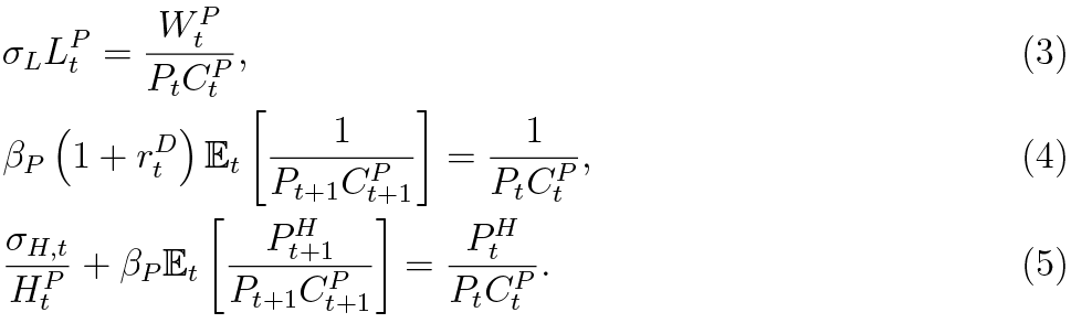
β_P is the household’s rate of time preference, λ_t^P is the Lagrange multiplier. Equation (3) states that, all else being equal, the household supplies more labour as real wages rise. Equation (4) is a standard Euler equation and (5) equalises marginal utility of housing to marginal disutility of foregone consumption when buying one unit of housing.

2.1.2. Impatient household

Although preferences are identical across households, the impatient has a more complex

problem to solve. Moreover, this agent is of particular interest from macroprudential perspective because it has the ability of taking out mortgages and defaulting on them. The defaulting framework used here is adopted from de Walque et al. (2010), which is an alternative to the more prevalent BGG setting (see e.g., Forlati and Lambertini, 2011; Darracq Pariès et al., 2011; Clerc et al., 2015). It is important to note that default rate is positive in the steady state, as well as off it.

The household earns labour income and is able to additionally borrow to finance consumption, service debt and accumulate housing asset. The debt service includes interest net of delinquencies, and coverage of default costs which consist of housing seizure and search costs. This is represented by the following budget constraint:

where W_t^I is the inpatient’s nominal wage rate, ΔL_t^H is change in stock of debt at the end of period t, is the predetermined² interest rate associated with t – 1 period debt. χ_t^H is an endogenous fraction of debt defaulted, Ω_t^H is search costs and S_t is bank asset seizure, both associated with period t – 1 default decisions.

Now we describe the latter three items in more detail. In this setting, a representative impatient household has full control of the default rate χ_t^H on previous period’s debt (). This fraction can also be interpreted as the share of individual household family members who have fully defaulted on their debt obligations. A virtue of this way of modelling is that the household does not automatically default on the basis of some specific rule, like in Bernanke et al. (1999), but takes into account all relevant variables and weighs the costs of default against the benefits.

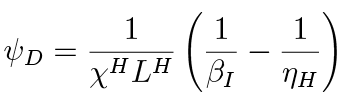
The search costs are understood as an inconvenience or rejected loan applications for the impatient household sector as a whole, resulting from past default decisions and worsening of credit score. The costs incurred at time t due to default at period t – 1 are:

Search costs are quadratic in the size of the default (), which ensures model stability. The parameter ψ_D controls the magnitude of the costs, and hence influences the willingness to default. In contrast to de Walque et al. (2010) specification, we do not find it necessary to include the (linear) default stigma costs in the instantaneous utility function, neither for model stability, nor for determinacy.

We assume that household’s borrowing from the banking sector is secured with housing. As usual, the household can borrow up to a certain limit which is a fraction of the nominal value of housing which serves as a collateral³. The standard borrowing limit, popularised by Kiyotaki and Moore (1997) and used in numerous papers with mortgages (e.g. Iacoviello, 2005; Gerali et al., 2010; Angelini et al., 2014) and mortgage defaults (e.g. Bekiros et al., 2017; Nookhwun and Tsomocos, 2017), is most suitable for one-period loans. However, introduction of multi-period loans can have an impact on monetary or macroprudential policy transmission mechanism (see e.g., Brzoza-Brzezina et al., 2014; Brzoza-Brzezina, 2014). Gelain et al. (2015, 2018) showed that multi-periodicity can be modelled using a stock mortgage variable entering the budget constraint conventionally, however, the borrowing limit should be an autoregressive version of the traditional Kiyotaki and Moore (1997) constraint. It has also been applied in Iacoviello (2015) and Chen and Columba (2016), among others. To account for multi-periodicity and more accurate loan dynamics, we use the following dynamic borrowing constraint:

where ρ coefficient controls the jumpiness of mortgage stock (L_t^H). The parameter approaches zero for one-period loans and unity for long term borrowing. η_t^H is an exogenous policy variable that we interpret as a LTV cap. The specification suggests that for multi period loans changes in LTV policy should have a prolonged impact. Long term mortgage stock to housing value ratio is equal to η_H .

Unlike in de Walque et al. (2010), we assume that any default would result in asset seizure by the bank. Otherwise, the collateral constraint would serve only as a limit on borrowing, and the word collateral would be meaningless in this context. The already mentioned models of Darracq Pariès et al. (2011) and Forlati and Lambertini (2011), Bekiros et al. (2017) and Nookhwun and Tsomocos (2017), have both BGG framework for mortgage default, and housing seizure.

In our model, any delinquency results in bank’s seizure of a fraction of household’s assets that is proportional to the size of the default rate. Under the baseline version of the model we assume that if a single household (family member) defaults on its debt, the bank seizes the whole house and sells it at the market value P_t^H . Since χ represents the share of households which defaulted in the past, the total asset seizure would be:

In normal times, when house prices are relatively stable, this type of asset seizure would incur large costs on the household because the nominal value of the seized house would be much higher than the defaulted amount. To see the point of this argument, let us assume for now that ρ = 0, and that the LTV constraint (8) holds with equality. Asset seizure at time t would be the following:

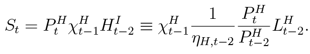
If we divide nominal size of asset seizure by the nominal amount defaulted, we have:

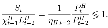
Using this equation, and ignoring search costs, one can see that if the house prices are falling by at least η_{H ,t–2}, the seized amount is lower than the amount defaulted. When house prices are falling less than η_{H ,t–2} or are stable/increasing, the seizure is relatively high compared to the amount defaulted, and the process is painful for the delinquent party. The household can still default wilfully because it is highly impatient (see Equation (13), where costs and benefits of default are compared). For alternative asset seizure specification, please see Subsection 4.2 and Appendix B. Judging from the equation above, one can see the virtue of the LTV limit at the origination. Smaller LTV implies a higher down payment for the household and makes asset seizure relatively large compared to the size of the default, thus protecting the bank. On the other hand, loose LTV is a concern for the bank because it makes the bank more susceptible to house price drops.

The impatient household chooses paths of C_t^I , L_t^I , H_t^I , L_t^H and default rate χ_t^H to maximise its expected discounted lifetime utility subject to the borrowing limit (8) and budget constraint (6). Optimisation results in the following conditions:

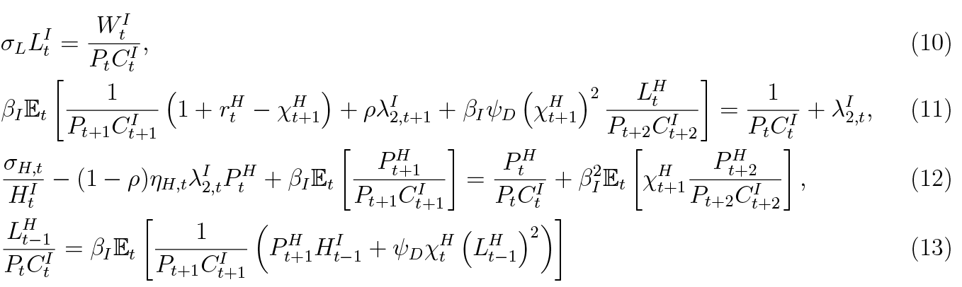
Labour supply equation (10) is no different from that of patient household’s. The Euler equation (11) takes discounted expected cost of borrowing, which consists of interest, debt repayment net of defaults and future search costs, and equates to marginal utility of additional consumption, taking into account the collateral constraint (). The housing demand equation (12) also has cost and benefit terms. On the benefit side of additional housing there is positive value from a looser borrowing constraint and positive future consumption in case of a resell if house prices increase. Note that high LTV limit (η_{H ,t}) increases the marginal utility coming from relaxation of the borrowing constraint. The cost side involves foregone current consumption and future loss of housing (two-periods ahead) in case of default. The last condition equates marginal utility of default, which allows the impatient household to increase immediate consumption, to a marginal cost, which is lost future housing and increased search costs.

The collateral constraint (8) is binding around the small neighbourhood of the steady state⁴ as long as β_P > η_H, presuming that shocks hitting the economy are sufficiently small.⁵

2.2. Firms

The firm sector is the same as in Karmelavicius and Ramanauskas (2019), being comprised of competitive producers of final goods and monopolistically competitive intermediate good producers. The homogeneous final goods are produced from intermediate goods and are suitable for both consumption and investment and can be used domestically or exported. The only difference from Karmelavicius and Ramanauskas (2019) is that the total labour employed by the intermediate producer is the following packaged index:

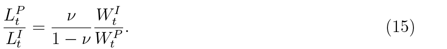
Cost minimisation of total labour expenditure 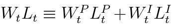gives the optimal labour demand ratio:

2.3. Banks

The modelled financial sector consists of a representative competitive foreign-owned bank. The model setting is similar to Karmelavicius and Ramanauskas (2019), except that banks also extend housing loans that can default and result in collateral seizure.

The bank has a stylised balance sheet comprised of two assets (loans to firms, L_t^F , and households), liabilities in the form of deposits and foreign debt (F_t), current profits (π_t^B ) and accumulated earnings (Π_t^B ):

Just like in the intermediate firm’s case, the bank’s balance sheet is expressed in nominal terms. Note that in this specification current quarter’s profits enter the balance sheet separately from bank accumulated earnings which is considered as regulatory capital⁶. The motion equation for bank capital is the following:

where DivB_t denotes endogenous bank dividends and is bank profits transferred from last period’s balance sheet. Assuming that bank dividends are non-negative, the bank may accumulate capital only from retained earnings; thus, external equity financing is assumed away for simplicity.

Our specification differs from other papers (e.g., de Walque et al., 2010; Gerali et al., 2010; Vītola and Ajevskis, 2011; Iacoviello, 2015; Pedersen, 2016) in at least three dimensions. Firstly, current quarter’s profits (π_t^B ) do not count as capital, in line with European regulation⁷, which stipulates that current quarter’s (unaudited) profits are not included in the regulatory capital. Secondly, all bank capital from the previous period is carried forward to current period, whereas abovementioned authors assume that a small fraction is used up for bank management. Thirdly, dividend stream is fully endogenous and at banker’s discretion in our model, whereas some authors assume that they are a fixed fraction of bank capital/equity.

The bank earns interest income on loans (corporate and household) and pays interest on deposits and foreign borrowing. Impatient household mortgage defaults reduce bank’s t period profits by but the bank is able to seize the impatient’s house as a collateral and sell it in the open market the next period t + 1 for , where o represents a fraction that is considered as administrative or monitoring costs such as bailiff fees⁸. All these items are reflected in the profit equation:

where r_t^H, r_t^L, r_t^D and r_t^F denote, respectively, nominal interest rates on loans (household and firm), deposits and banks’ foreign debt. Note that the specification of the bank profit function implies that today’s net interest income is determined by yesterday’s decisions, which reflects the intertemporal nature of bank’s finance.

The last term in the bank’s profit equation is income after asset seizure, resulting from previous mortgage defaults, thus not influenced by the bank (see Subsection 2.1.2 for more details). Since the collateral constraint (8) of the impatient household is binding, the bank is aware of that. Therefore, we plug the LTV constraint in place of in the profit equation:

Now it is evident that banks are aware that past lending might influence profitability through defaults and asset seizure. If house prices are falling, and especially when the rate of fall is bigger in magnitude than 1 – η_{H ,t – 2}, the defaults can be very dangerous to bank profitability, because the collateral is not enough to cover the losses. The administrative cost parameter o is calibrated so that the bank would not profit off asset seizure in a stable house price environment.

Most authors tend to include LTV constraint in the optimisation of the borrowing party, as we did. However, the expanded profits specification above suggests that LTV caps directly influence banker’s optimisation problem, and thus credit supply, which will be evident in later simulations.

Before we move to optimisation, a couple of other assumptions should be stated. Firstly, the banks are owned by a foreign-based banker who is a hand-to-mouth consumer and finances her foreign consumption with dividend payouts. Secondly, although the model in its form does incorporate household credit default risk, that does not imply that a significant share of bank financing should come in the form of equity. In order to institute positive bank equity we assume that the banker receives utility from increasing bank capital buffer over the regulatory minimum. Below is the banker’s instantaneous utility function:

where C_t^* is banker’s foreign consumption and Ω_t^B is a utility term that captures the benefit of excess bank capital. We specify the latter as a logarithmic function as in Furfine (2001):

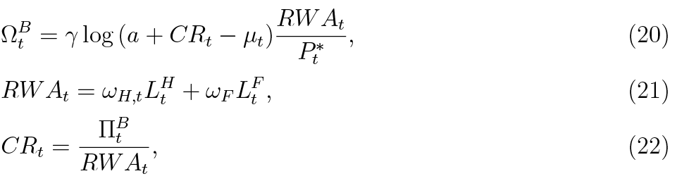
where C R_t is the (regulatory) capital adequacy ratio, μ_t is the minimum requirement, RW A_t denotes risk-weighted assets, ω_H,t and ω_F are exogenous risk weights. γ is the parameter reflecting the utility associated with a capital buffer.

We also specify the upward sloping foreign financing supply function, similar to Schmitt-Grohé and Uribe (2003). It states that the interest rate on banks’ foreign debt positively depends on the nominal foreign debt-to-GDP ratio:

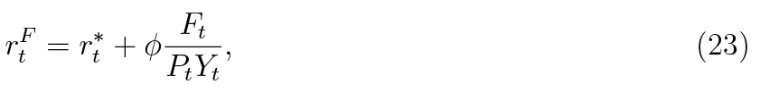
where r_t^* is the risk-free interest rate on borrowing in foreign financial markets and φ is a non-negative parameter that controls the risk premium.

Maximising banker’s discounted lifetime utility with respect to paths of π_t^B, Div B_t, L_t^H, L_t^F, F_t and Π_t^B yield the following first-order conditions:

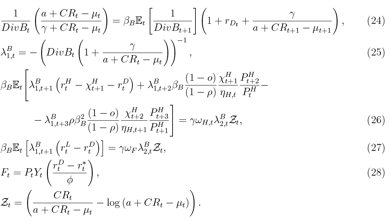
There is a close analogy between the banker’s Euler equation (24) and the household’s Euler equation (4). The banker equates the marginal rate of substitution between dividends today and tomorrow to the relative price of dividend pay-outs. Expansion of bank capital reduces the alternative cost of deposit-financing and increases marginal utility stemming from wider capital buffer.

Equations (26) and (27) establish that bank’s capital buffers are increasing with an increasing interest rate margin. What is more, mortgage supply rule (26) states that interest rates are higher when expectations for future defaults, net of asset seizure, increase. Tight collateral constraint or expectations of house price growth suppress the mortgage interest rate margin. Equation (28) governs demand for foreign debt, which is positive when deposit rates are higher than the risk-free rate. Also, all else being equal, the lower risk-free foreign rate naturally implies stronger demand for bank’s borrowing from abroad.

2.4. Closing equations

Adding the households’ budget constraints together with the firm’s and bank’s balance-sheet constraints, we obtain the following identities

where NX_t is the net exports. Equation (29) is simply an aggregate resource constraint. Equation (30) is the simplified balance-of-payments identity, which states that the combined current and capital account, comprised of net exports and net financial income from abroad in this simple economy, must equal the financial account, or in this case simply the change in foreign debt. The nominal gross domestic product is defined as output net of firm’s adjustment costs, household’s search costs and bank’s foreclosure costs:

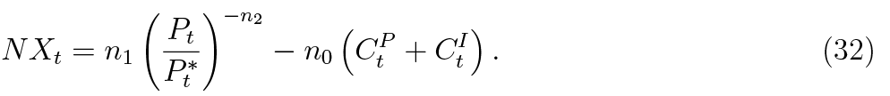
Since monetary policy is absent from this economy, Taylor rule is unavailable. Therefore, a closing equation is necessary to be able to identify the price level, as in Aoki et al. (2018). We assume that the domestic price level is determined by an external competitiveness condition which relates net exports to the the real exchange rate and domestic consumption:

A very similar approach is taken by Vītola and Ajevskis (2011) in their model of the Latvian economy, as well as Aoki et al. (2018. We assume there is no inflation in foreign economy:

The supply of housing is fixed, which implies the following clearing condition:

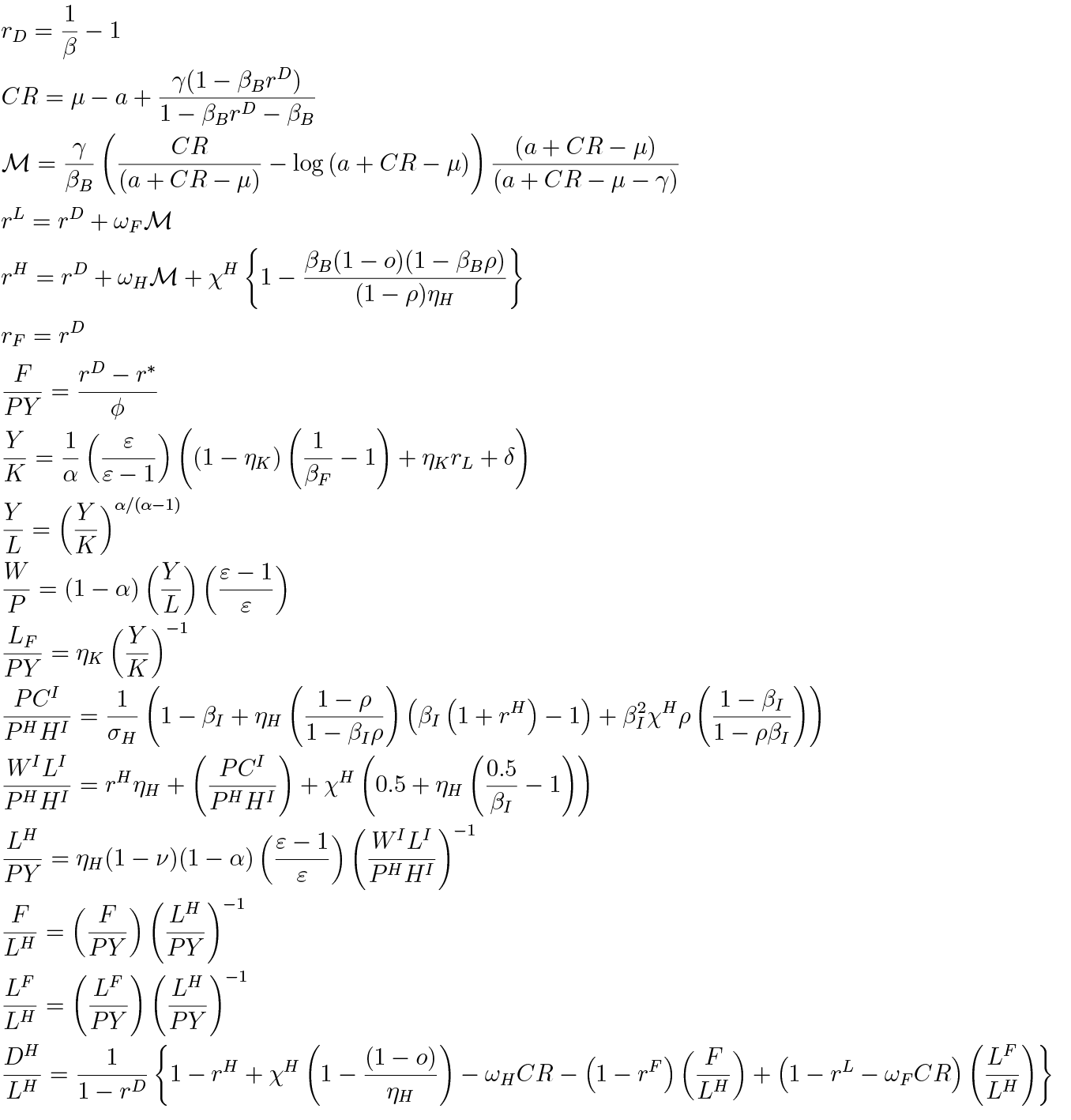
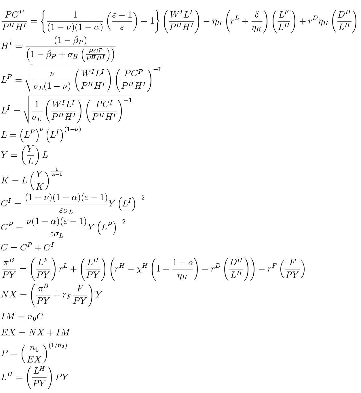
A full list of model equations is presented in Appendix C.

3. Calibration

We calibrate the model’s parameters to match some general macroeconomic ratios of the Lithuanian economy at quarterly frequency for the period 2004-2018. The matched first moments of the data are tabulated in Table 1, and chosen parameter values are presented in Table 2. The numerical values for α, β_F, δ, and ηK are chosen simultaneously to produce the following steady state ratios: corporate loans to annual GDP ratio of 24%, investment to GDP ratio of 21%, the capital share in aggregate income of 31%⁹ and firms’ return on equity of 8%, in line with the corresponding historical averages in Lithuania. The value of ε = 34, was chosen so that the β_F would be sufficiently low in the (simultaneous) calibration exercise, which would imply a binding firm collateral constraint. The elasticity of demand for intermediate goods constitutes a mark-up of 3%.

Table 1. Matched steady state ratios (annualised).

Variable	Interpretation	Value (%)
L / PY	Corporate debt to GDP ratio	24
I / Y	Investment share	21
WL / PY	Labour compensation share	69
π / Π	Firm’s ROE	8.2
rD	Interest rate on deposits	1.2
LH / PHHI	Loan to collateral ratio (average)	78
LH / PY	Mortgage debt to GDP ratio	16
χH	Mortgage non-performing loans ratio	5
μ	Bank capital requirement (average)	14.5
CR	Bank capital adequacy ratio	19
rH	Interest rate on mortgages	3.4
rL	Interest rate on firm loans	3.9
πB / (πB + ΠB)	Banks’ ROE	10
r*	Risk-free interest rate	1.06
F / PY	Bank net external debt to GDP ratio	12

The investment adjustment cost parameter ψ_I = 2.65 is taken from the Bayesian mean estimate in Vītola and Ajevskis (2011). The price adjustment cost parameter ψ_P = 380 in our model would correspond to a 75% chance that prices will remain unchanged in a given quarter – a typical probability in models with Calvo pricing.

The patient household’s discount factor β = 0.987 corresponds to the historical average nominal interest rate on private sector deposits (including both sight and term deposits) of 1.3%. ν = 0.75 is chosen to approximate the share of impatient households to be around 25%, in line with historical share of housing purchases financed with bank debt. η_H = 0.78 is equal to the historical average LTV of new housing loans. ρ = 0.7is taken from Iacoviello (2015) which ensures that mortgages are a slow moving variable, with average maturities over 20 years. σ_H is consistent with mortgage debt to annual GDP ratio of 16% and σ_L ensures that impatient’s labour is equal to unity in the steady state. β_I = 0.75 chosen sufficiently low to ensure that the LTV constraint is binding and household default rate is positive. ψ_D = 2.537 corresponds to an average mortgage NPL rate of 5% in Lithuanian banking sector.

Table 2. Parameter values.

Parameter	Description	Value
α	Capital share in the production	0.29
δ	Depreciation rate for physical capital	0.039
ηK	Loan to value cap for firms loans	0.18
βF	Firm management’s discount factor	0.986
ε	Price elasticity of demand for intermediate goods	34
ψP	Price adjustment costs parameter	380
ψI	Investment adjustment costs parameter	2.65
βP	Patient household’s discount factor	0.997
ν	Patient household’s share of labour income	0.75
ηH	Housing loans to collateral value ratio	0.78
ρ	Autoregressive coefficient in mortgage LTV equation	0.7
σH	Utility from housing	0.66
σL	Disutility from labour	1.05
βI	Impatient household’s discount factor	0.75
ψD	Size of quadratic default search costs	2.537
μ	Minimum capital requirement	0.145
a	Parameter controlling the excruciating bank capital level	0.085
ωH	Risk weight on mortgages	0.5
ωF	Risk weight on corporate loans	1.55
γ	Banker’s utility from capital buffer	1.212 × 10–3
o	Mortgage monitoring costs	0.44
βB	Banker’s discount rate	0.988
φ	Foreign debt interest rate sensitivity	7.291 × 10–3
n0	Imports to consumption share	0.9
n1	Constant exports demand	1.8
n2	Price elasticity of exports demand	1

Minimum bank capital requirement parameter μ = 0.145 corresponds to recent value of average capital requirements for banks in Lithuania (including Pillar I and Pillar II capital). Value of α = 0.085 was chosen so that the excruciating capital ratio would be associated with 6%. These are roughly Basel 2 type capital requirements excluding capital buffers and additional individual bank requirements. ω_H = 0.5 is consistent with historical average risk weight on mortgages in Lithuania’s banking sector. We jointly calibrate parameter values of ω_F, γ, o and β_B to produce capital ratio of 19%, average mortgage interest rate of 3.4%, corporate debt interest rate of 3.9% and bank ROE of 10%. The latter three ratios correspond to Lithuanian data averages, and capital ratio of 19% is a recent level of capitalisation in the banking sector. Foreign financing supply φ is calibrated to make bank’s net foreign debt to GDP ratio equal to 12%.

Turning to the parameters related to the foreign trade, the parameter n₀ = 0.9 reflects the historical average imports to consumption ratio in Lithuania. As there is little empirical evidence about the long-term equilibrium level of trade balance, we arbitrarily choose the parameter n₁ to ensure that in the steady state there is a small trade surplus, which would offset financial outflows in the form of bank dividends and interest rate payments on foreign debt (resulting in the balanced current account in the steady state). The value of the parameter n₂, governing the price elasticity of exports, is set equal to 1, like in Vitola and Ajevskis (2011).

4. Analysis and results

This section is devoted to the analysis of the short term impact of tightening of three prudential policy instruments, namely, the bank capital requirement, mortgage risk weight and cap on loan to value for mortgages.

4.1. Some steady state conditions

In this subsection we take a look at some of the analytically derived steady states from the banker’s problem, to understand what determines the capital ratio and interest rate on loans in the long term. Although this comparative statics exercise is done for the steady state, it sheds light on the short-run dynamics as well. The steady state bank capital adequacy ratio can be expressed as:

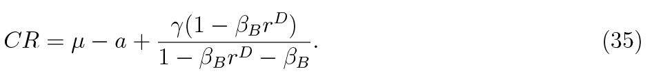
It is visible that in the steady state the capital ratio (CR) increases one-to-one with the regulatory minimum μ. The excess capital buffer (CR – μ) positively depends on the deposit interest rate r^D, which is the cost of debt financing. Rising banker’s impatience, roughly the opportunity cost of accumulating bank capital, decreases the CR (βF ↓ ⇒ CR↓). This can be understood as rising returns outside the banking sector, which decrease the willingness to hold more bank capital.

Although the CR is calculated as the ratio of capital to risk weighted assets, the steady state CR is independent of the risk weights. However, risk weights (ω_F, ω_H) can be understood as capital intensity of each asset type affecting portfolio allocation and interest rates. The steady state interest rates of corporate and mortgage loans can be expressed as:

with being overall cost of equity. We see that in the latter two pricing equations, risk weights act as loan-specific linear transformations from the cost of equity to interest rates. When a risk weight of a certain type of loan rises, that loan becomes more capital-intensive, which translates into higher capital costs and thus interest rates.

The interest rate on corporate loans is a sum of cost of debt (r^D) and cost of equity (ω_F), whereby the mortgage rate also includes the risk premium. One can see that when mortgage delinquencies (χ^H) rise in the steady state, the interest rates are incremented less than 1-to-1. This is because after a delinquency occurs, the bank is able to seize household’s collateral and sell it in the open market. Careful inspection of the risk premium suggests that when administrative or monitoring costs (o) rise, bank’s net losses are greater, so the premium is higher. Given the baseline assumption that the bank seizes the whole house (see discussion in Subsections 2.1.2 and 2.3), in case of mortgage delinquency and absent monitoring costs (o = 0), the bank can profit in stable house price environment. The size of monitoring costs is calibrated so that the bank wouldn’t profit from asset seizure, and that the risk premium would be positive.

Interestingly, the cap on loan to value ratio (η_H) is also present in the pricing equation (37). This result, as can be seen in later simulations, is implied by the banker’s awareness that high collateral seizure is associated with past loose lending. When collateral constraint becomes tight, the household has to use more own-funds for a house purchase, therefore the bank becomes more covered in a case of default. As a result of the increased banker’s protection, the mortgage riskiness decreases and thus the interest rate is lower. It implies that the LTV limit has a direct impact on the credit supply. While a tight constraint has a positive effect on the supply, a loose constraint can leave the bank vulnerable to asset price drops, and thus contributes negatively to the credit supply.

Using the formulas above, the mortgage spread can also be expressed in this convenient fashion:

where one could see that mortgage spreads and corporate spreads are positively related. As in a typical problem of portfolio management, corporate loan rate can be considered as an opportunity cost of allocating funds towards mortgages. Any increase in the profitability of corporate lending should reduce the mortgage supply and increase the rates thereafter. The sensitivity of this pass-through is defined by the ratio of mortgage to corporate risk weights. The more mortgages are capital intensive, compared to corporate loans, the greater the pass-through from higher corporate returns, all else being equal.

4.2. LTV tightening

Here we take a look at the model’s responses to a permanent decrease in LTV limit by 1 p.p. This can be understood as a reduction in the regulatory risk appetite in order to safeguard the debtors and lenders. LTV constraint is usually understood as a demand-side-only constraint, entering borrower’s optimisation (see e.g., Kiyotaki and Moore, 1997; Iacoviello, 2005; Gerali et al., 2010; Justiniano et al., 2015). Using the baseline asset seizure assumption, we show that a tightening of LTV limit has non-negligible credit supply-side impact.

Model variable responses to a permanent LTV tightening by 1 p.p. are shown as pale blue lines in Figure 2 of Appendix A. There are three important developments related to household mortgages. Firstly, when an LTV cap is lower, the impatient household has comparatively more to lose when defaulting on a mortgage, thus the default rate decreases by around 1.75% over 5 years. Qualitatively, a similar response has been found in micropanel studies of González et al. (2016), Mihai et al. (2018) and Gaudêncio et al. (2019). Secondly, there is a significant reduction in interest rates on mortgages by 0.3 to 0.6 p.p. Thirdly, lending decreases immediately by 0.5%, followed by a peak decline of around 2% in the medium term and then 0.5% again in 5 years.

Both interest rate and lending fall suggesting of a dominant negative demand channel in the shock propagation mechanism. However, the banker, when optimising, takes into account both household default rate and the LTV (see equations (26) and (37)). Both these factors make housing loans a safer investment from bank’s perspective. Lower loan to value ratio implies that a bank loses less after a default happens, but also the household default rate is decreased. This contributes to an increase in mortgage supply which reinforces the drop in interest rate (lower margins) but attenuates the negative response in mortgage loans.

Lending to the corporate sector also decreases by around 0.1% in 5 years with interest rates being more or less the same. With regards to house prices, they decrease nominally by around 0.15% and in real terms by around 0.1%. Overall, there is a negative impact on GDP in 4 years being around 0.1%, which exactly coincides with results obtained by Richter et al. (2018). Since there is a general drop in economic activity and prices, we would characterise such tightening of requirements as a net drag on mortgage demand and aggregate demand.

4.3. Tightening of bank-based measures

While the limit on loan to value ratio is considered to be a borrower-based instrument, bank capital requirements and risk weight floors are bank-based measures. In our model the LTV limit is internalised in the decision making of both the bank and the borrower, whereas the bank-based measures are not taken into account when optimising by the impatient household.

4.3.1. Bank capital requirements

In this subsection we do not differentiate between different capital add-ons or buffers. We assume that a regulatory authority requires all banks to permanently hold 1 p.p. higher capital ratio. The responses of our model economy are depicted in Figure 4 of Appendix A.

Accumulation of resources in the form of bank capital implies an opportunity cost in terms of foregone consumption for the owners, what directly translates into higher interest rates on bank loans. Firm rates respond smoothly, being 0.12-0.15 p.p. higher. The response of mortgage rates is relatively more pronounced in the beginning with 0.07 p.p. and normalises to 0.03 p.p. in 5 years. The short-term estimate is close to 0.095 p.p. estimate for commercial real estate loans of Glancy and Kurtzman (2018), where authors used micro level data. The reason why these two rate reactions differ is the increase in mortgage default rate in the medium term, which shows up as a higher mortgage risk premium. Overall, interest rate on firm loans increases more because the latter type bears higher risk weight than household loans.

While both types of lending contract by a similar amount of 0.2% in the longer term, corporate loans do decrease more than mortgages in the short run. This finding has been established in several other bank panel (e.g. Budrys et al., 2017; Mayordomo and Rodriguez Moreno, 2018) and multivariate time series (e.g. Noss and Toffano, 2016; Kanngiesser et al., 2017) studies. An important source of this difference is that risk weights for corporate exposures are usually higher than those of mortgages. We also see that, as the bank is deleveraging, it reduces the amount of deposits (and foreign financing) and is able to steadily accumulate bank regulatory capital, even with higher dividend payouts. Higher dividend payouts are possible because of higher profits, which result from higher interest rate margins. The result that capital requirements can increase bank profitability is visible also in models of of Gerali et al. (2010) and Vītola and Ajevskis (2011). When higher capital requirements are implemented for an individual bank, a response by raising interest margins would produce a loss in demand and therefore profitability. However, when capital requirements are applied for the sector as a whole, all banks increase their margins at the same time and thus can be more profitable.

With regards to the general macroeconomy, we see that responses of house prices and consumption are modest compared to that of investment, because corporate lending and its margins react more severely. Although the nominal house prices deflate, they do not go down as much as the general price level, making real house prices grow for some time. The impact on GDP is small and equal to around -0.02% in the short term and around -0.04% in the medium term. Judging from variable response, a tightening of bank capital requirements can be thought of as a negative credit supply shock (increased rates, reduced lending, e.g. see Justiniano et al., 2015) which traslates into a negative drag on aggregate demand (reduction in output and deflation).

4.3.2. Mortgage risk weight

Bank asset risk weights in reality are endogenous variables that move over time in response to bank’s assessment of the underlying riskiness of its assets. Usually, as the economy expands, the perception of risk decreases, thus making risk weights counter-cyclical. Recent data shows (see Bruno et al., 2017) that after the financial crisis the risk weights of assets have been moving downwards, especially of those banks that use the internal ratings based (IRB) method. For a regulator this can cause a concern, whether these trends truly reflect the underlying asset riskiness. European Capital Requirements Regulation Art. 458 allows designated national authorities to exercise national flexibility measures and implement a floor for risk weights for a particular type of assets like mortgages. For some banks this floor might be binding, essentially raising the average risk weight (risk weight density) prevailing in the market for mortgages.

We implement a simulation of the model where risk weights on mortgages are raised by 5% (or 2.5 p.p. under baseline calibration) indefinitely. Such action increases overall risk-weighted assets, requiring more bank capital to keep the capital ratio constant. Special treatment of mortgage risk weights induces the latter asset class to be more capital-expensive. The model variable simulations are produced in Figure 5 of Appendix A. We see that mortgage interest rates rise by around 0.04 p.p. in 5 years. This estimate is very close to the micro data based estimate of 0.035 p.p. by Glancy and Kurtzman (2018)¹⁰. Regarding loan portfolio, corporate loans fall by up to 0.01% and mortgages by up to 0.1%. This clearly shows that there is a negative supply side shock in loans market, and a reshifting of bank portfolio towards corporate loans. Tight conditions in the mortgage market coupled with increased interest rates lead to a minuscule increase in household mortgage defaults. As in the case of tightening of capital requirement, the banking sector substitutes debt financing towards equity financing, as bank regulatory capital grows and leverage decreases. Also, the banking industry as a whole is able to accumulate capital even with increased bank dividends, resulting from higher profitability due to higher interest margins.

Like capital requirements, mortgage risk weight brings down the nominal house and goods prices in the economy, but overall deflation is higher than that of housing, leaving real house prices a bit higher. Since negative lending supply shock is a drag on domestic demand (consumption and investment), wee see the prices falling and through net exports increase. Although real GDP falls initially, it picks up in the medium term due to increased exports. All in all, the effects of changing mortgage risk weights are rather minuscule, as can be seen from the next subsection.

4.4. Comparison of effectiveness in taming household credit growth

Previous simulations show that all three instruments when tightened, can have negative impact on credit, mortgages and economic activity. Bank capital regulation is intended to safeguard banks against credit losses, which are a risk that can be of structural and cyclical nature. However, there can be an incentive for a regulator to use, for example, bank capital regulation for mortgage market stabilisation purposes. Demanding more bank capital might have unintended consequences for the economy and especially for the production sector. In this subsection, we compare the impact of the three prudential measures on the mortgage market and the general economy. To this end, we perform a simulation, in which all measures are separately tightened on a permanent basis. For the results to be comparable, we induce requirement changes so that the peak negative impact on credit market is equivalised to 0.1%. The resulting changes are depicted in Figure 6 of Appendix A.

One can immediately notice that tightening of capital requirements has the biggest negative drag on firm credit supply, i.e. the reaction of interest rate and credit is stock is the highest. This reduction in availability of funding leads to highest losses in output, compared to other scenarios. Increases in mortgage risk weights have the smallest impact on corporate debt credit market. These response functions indicate that broad-based capital requirements is the least suitable instrument of the triplet for reducing mortgage growth, because it has non-negligible distortionary effect on production sector. Risk weight management and tightening of LTV limits seem like the more viable option for leaning against, for instance, unsustainable growth in the mortgage market. Capital requirements, e.g. the countercyclical capital buffer, can be better used as a tool address broad-based risks arising in the whole financial sector, not limited to some specific sector. The sectoral countercyclical capital buffer would be a more effective tool in dealing with cyclical risks that are of confined to a specific sector.

5. Concluding remarks

After the financial crisis of 2009 macroprudential policy arose as a new systemic approach to mitigate risks and enhance the resilience of the financial sector. Since the policy tool-set is still relatively new, empirical impact estimation is complicated. DSGE models, featuring financial frictions, can be a useful tool to understand the nature of the past financial crisis as well as predict the possible impact of the new regulatory instruments and their interaction.

We built and calibrated a small open economy DSGE model with banking and two-sector lending for Lithuania. The model features household mortgages that are risky from bank’s perspective, and thus are collateralised with housing, which can be seized after a delinquency. Following Iacoviello (2015) and Gelain et al. (2015, 2018), mortgage dynamics reflect that of multi-period loans, what is an improvement over general models that feature household default. It is assumed that the bank is aware of the collateral constraint and asset seizure when making lending decisions, thus making the LTV limit also a supply-side factor, in addition to the traditional demand-side constraint.

We simulate a tightening of three macroprudential policy measures, namely the LTV cap, bank capital requirement and risk weights, and assess their impact. A 1 p.p. point tightening in the mortgage LTV requirement reduces housing interest rates by a rather large 0.3 p.p. due to an expansion of credit supply which exacerbates the effect of reduced loan demand. The impact on lending is around -0.5% and -0.1% on GDP, similar to Richter et al. (2018) and Reichenbachas (2020).

An increase in bank capital requirements by 1 p.p. increases interest rates on corporate lending by 0.12 p.p. and on mortgages by 0.03 p.p., which is similar to estimates based on ad hoc formulas used by banks. The impact on general lending is only 0.2 p.p., however, corporate lending tends to be cut more in the short-term. This result stems from the fact that loans to businesses tend to carry higher risk weights, and is consistent with other studies (such as Budrys et al., 2017; Mayordomo and Rodriguez-Moreno, 2018). As per increased regulation of risk weights by 5% (or 2.5 p.p.), mortgage interests rates rise by 0.04 p.p. as in Glancy and Kurtzman (2018) and lending decreases by 0.1 p.p.

After a comparison of different macroprudential policy tools for leaning against the wind in the mortgage market, we find that broad-based capital requirement is less effective and does more harm to the corporate sector and the economy as a whole. More targeted tools as cap on LTV and risk weight regulation can produce a better effect when the objective is to target risks in housing market. Therefore, instruments such as the counter-cyclical capital buffer are suboptimal in times when cyclical risks are building up only in the mortgage sector.

References

Angelini, P., Neri, S., and Panetta, F. (2014). The interaction between capital requirements and monetary policy. Journal of Money, Credit and Banking, 46(6):1073–1112.

Aoki, K., Benigno, G., and Kiyotaki, N. (2018). Monetary and financial policies in emerging markets. Manuscript available.

Bekiros, S. D., Nilavongse, R., and Uddin, G. S. (2017). Mortgage defaults, expectation-driven house prices and monetary policy. Economics Working Papers ECO 2017/09, European University Institute.

Bernanke, B., Gertler, M., and Gilchrist, S. (1999). The financial accelerator in a quantita- tive business cycle framework. In Taylor, J. B. and Woodford, M., editors, Handbook of Macroeconomics, volume 1, Part C, chapter 21, pages 1341–1393. Elsevier.

Bruno, B., Nocera, G., and Resti, A. (2017). The impact of risk-based capital requirements on corporate lending: Evidence from Europe. Discussion paper DP12007, Centre for Economic Policy Research.

Brzoza-Brzezina, M. (2014). Financial frictions and macroprudential policy. International Journal of Central Banking, 10(2):249–261.

Brzoza-Brzezina, M., Gelain, P., and Kolasa, M. (2014). Monetary and macroprudential pol- icy with multiperiod loans. NBP Working Papers 192, Narodowy Bank Polski, Economic Research Department.

Budrys, Z., Cappelletti, G., Marques, A. P., and Varraso, P. (2017). Macroprudential policy, O-SII bank capital buffers and their effects: Evidence from the euro area experiments.

Chen, J. and Columba, F. (2016). Macroprudential and monetary policy interactions in a DSGE model for Sweden. IMF Working Papers 16/74, International Monetary Fund.

Christiano, L. J., Eichenbaum, M. S., and Trabandt, M. (2018). On dsge models. Journal of Economic Perspectives, 32(3):113–40.

Claessens, S., Kose, M. A., and Terrones, M. E. (2009). What happens during recessions, crunches and busts? Economic Policy, 24(60):653–700.

Clancy, D. and Merola, R. (2017). Countercyclical capital rules for small open economies. Journal of Macroeconomics, 54(PB):332–351.

Clerc, L., Derviz, A., Mendicino, C., Moyen, S., Nikolov, K., Stracca, L., Suarez, J., and Vardoulakis, A. P. (2015). Capital regulation in a macroeconomic model with three layers of default. International Journal of Central Banking, 15(3):9–63.

Crowe, C., Dell’Ariccia, G., Igan, D., and Rabanal, P. (2013). How to deal with real estate booms: Lessons from country experiences. Journal of Financial Stability, 9(3):300–319.

Darracq Pariès, M., Kok Sørensen, C., and Rodriguez-Palenzuela, D. (2011). Macroeconomic propagation under different regulatory regimes: Evidence from an estimated DSGE model for the Euro Area. International Journal of Central Banking, 7(4):49–113.

de Walque, G., Pierrard, O., and Rouabah, A. (2010). Financial (in)stability, supervision and liquidity injections: A dynamic general equilibrium approach. The Economic Journal, 120(549):1234–1261.

Dellas, H., Diba, B., and Loisel, O. (2010). Financial shocks and optimal policy. Working papers, Banque de France.

Forlati, C. and Lambertini, L. (2011). Risky mortgages in a DSGE model. International Journal of Central Banking, 7(1):285–335.

Furfine, C. (2001). Bank portfolio allocation: The impact of capital requirements, regulatory monitoring, and economic conditions. Journal of Financial Services Research, 20(1):33–56.

Gaudêncio, J., Mazany, A., and Schwarz, C. (2019). The impact of lending standards on default rates of residential real estate loans. Occasional Paper Series 220, European Central Bank.

Gelain, P., Lansing, K. J., and Natvik, G. J. (2015). Leaning against the credit cycle. Working Paper 2015/04, Norges Bank.

Gelain, P., Lansing, K. J., and Natvik, G. J. (2018). Leaning against the credit cycle. Journal of the European Economic Association, 16(5):1350–1393.

Gerali, A., Neri, S., Sessa, L., and Signoretti, F. (2010). Credit and banking in a DSGE model of the euro area. Journal of Money, Credit and Banking, 42(S1):107–141.

Gertler, M. and Kiyotaki, N. (2015). Banking, liquidity, and bank runs in an infinite horizon economy. American Economic Review, 105(7):2011–43.

Glancy, D. P. and Kurtzman, R. J. (2018). How do capital requirements affect loan rates? Evidence from high volatility commercial real estate. Finance and Economics Discussion Series 2018-079, Board of Governors of the Federal Reserve System (US).

González, L., Durán Santomil, P., Lado Sestayo, R., and Búa, M. (2016). The impact of loan- to-value on the default rate of residential mortgage-backed securities. The Journal of Credit Risk, 12:1–13.

Goodhart, C., Tsomocos, D., and Shubik, M. (2013). Macro-Modelling, Default and Money. FMG Special Papers sp224, Financial Markets Group.

Goodhart, C. A. E. and Tsomocos, D. (2011). The role of default in macroeconomics. IMES Discussion Paper Series 11-E-23, Institute for Monetary and Economic Studies, Bank of Japan.

Guerrieri, L. and Iacoviello, M. (2017). Collateral constraints and macroeconomic asymmetries. Journal of Monetary Economics, 90(C):28–49.

Hoon Lim, C., Costa, A., Columba, F., Kongsamut, P., Otani, A., Saiyid, M., Wezel, T., and Wu, X. (2011). Macroprudential Policy; What Instruments and How to Use them? Lessons From Country Experiences. IMF Working Papers 11/238, International Monetary Fund.

Iacoviello, M. (2005). House Prices, Borrowing Constraints, and Monetary Policy in the Busi- ness Cycle. American Economic Review, 95(3):739–764.

Iacoviello, M. (2015). Financial Business Cycles. Review of Economic Dynamics, 18(1):140–164.

Iacoviello, M. and Neri, S. (2010). Housing market spillovers: Evidence from an estimated DSGE model. American Economic Journal: Macroeconomics, 2(2):125–64.

Jordà, O., Schularick, M., and Taylor, A. M. (2013). When credit bites back. Journal of Money, Credit and Banking, 45(s2):3–28.

Jordà, O., Schularick, M., and Taylor, A. M. (2017). Macrofinancial history and the new business cycle facts. NBER Macroeconomics Annual, 31(1):213 – 263.

Justiniano, A., Primiceri, G. E., and Tambalotti, A. (2015). Credit supply and the housing boom. NBER Working Papers 20874, National Bureau of Economic Research.

Kanngiesser, D., Martin, R., Maurin, L., and Moccero, D. (2017). Estimating the impact of shocks to bank capital in the euro area. Working Paper Series 2077, European Central Bank.

Karmelavičius, J. and Ramanauskas, T. (2019). Bank credit and money creation in a DSGE model of a small open economy. Baltic Journal of Economics, 19:296–333.

Karpavičius, S. (2008). Calibrated DSGE model for the Lithuanian economy. Pinigų studijos (Monetary Studies), Nr. 2:22–46.

Kiyotaki, N. and Moore, J. (1997). Credit cycles. Journal of Political Economy, 105(2):211–248. Lozej, M., Onorante, L., and Rannenberg, A. (2017). Countercyclical capital regulation in a small open economy dsge model. Research Technical Papers 03/RT/17, Central Bank of Ireland.

Mayordomo, S. and Rodriguez-Moreno, M. (2018). How do european banks cope with macro-prudential capital requirements?

Mihai, I., Popa, R., and Banu, E. (2018). The probability of default for private individuals using microeconomic data. What is the role played by macroprudential measures? Link to manuscript.

Nookhwun, N. and Tsomocos, D. (2017). Mortgage default, financial disintermediation and macroprudential policies.

Noss, J. and Toffano, P. (2016). Estimating the impact of changes in aggregate bank capital requirements on lending and growth during an upswing. Journal of Banking & Finance, 62(C):15–27.

Pedersen, J. (2016). An estimated DSGE-model for Denmark with housing, banking, and financial frictions. Danmarks Nationalbank Working Paper No. 108.

Proškutė, A. (2012). Business cycle drivers in Lithuania. Pinigų studijos (Monetary Studies), Nr. 1:5–29.

Quint, D. and Rabanal, P. (2014). Monetary and macroprudential policy in an estimated DSGE model of the Euro Area. International Journal of Central Banking, 10(2):169–236.

Reichenbachas, T. (2020). Assessing the impact of macroprudential measures: The case of the LTV limit in Lithuania. Bank of Lithuania Working Paper Series 80, Bank of Lithuania.

Richter, B., Schularick, M., and Shim, I. (2018). The costs of macroprudential policy. Working paper 24989, National Bureau of Economic Research.

Schmitt-Grohé, S. and Uribe, M. (2003). Closing small open economy models. Journal of International Economics, 61(1):163–185.

Townsend, R. M. (1979). Optimal contracts and competitive markets with costly state verifi- cation. Journal of Economic Theory, 21(2):265–293.

Vītola, K. and Ajevskis, V. (2011). Housing and banking in a small open economy DSGE model. Working Papers 2011/03, Latvijas Banka.

Vlcek, J. and Roger, S. (2012). Macrofinancial Modeling At Central Banks; Recent Develop- ments and Future Directions. IMF Working Papers 12/21, International Monetary Fund.

A. Figures

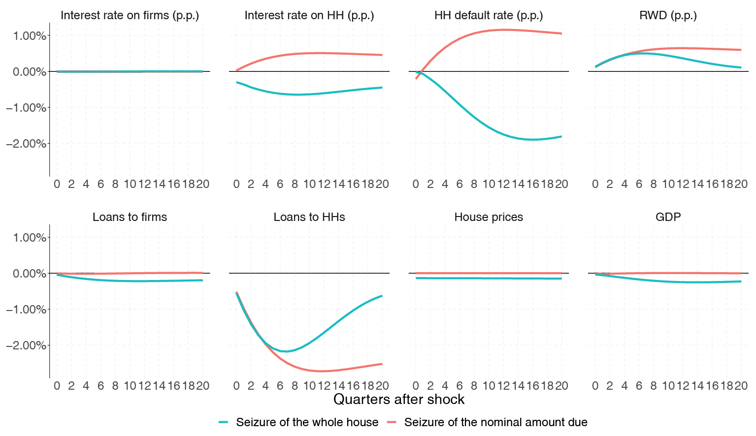
Figure 2. Comparison of responses to an unexpected and permanent rise tightening of LTV constraint by 1 p.p. under the baseline assumption of seizure of whole house, and alternative assumption of recovery of amount defaulted.

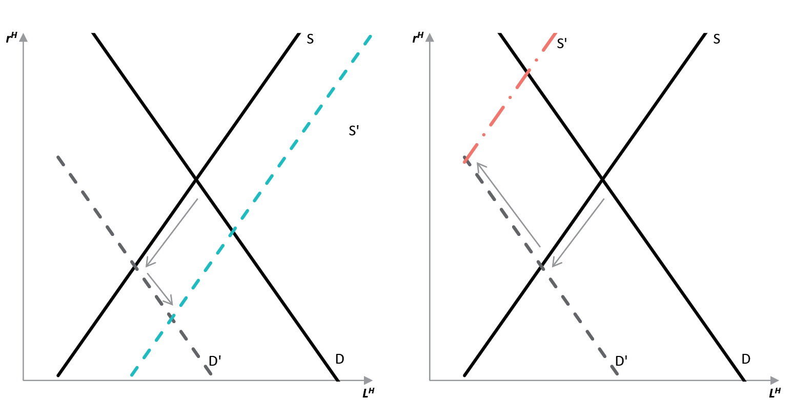
Figure 3. Stylised depiction of changes in credit supply and demand after LTV tightening occurs. Under the assumption of seizure of whole house (left), and bank recovery of the whole amount defaulted (right). Stylised depiction of changes in credit supply and demand after LTV tightening occurs. Under the assumption of seizure of whole house (left), and bank recovery of the whole amount defaulted (right).

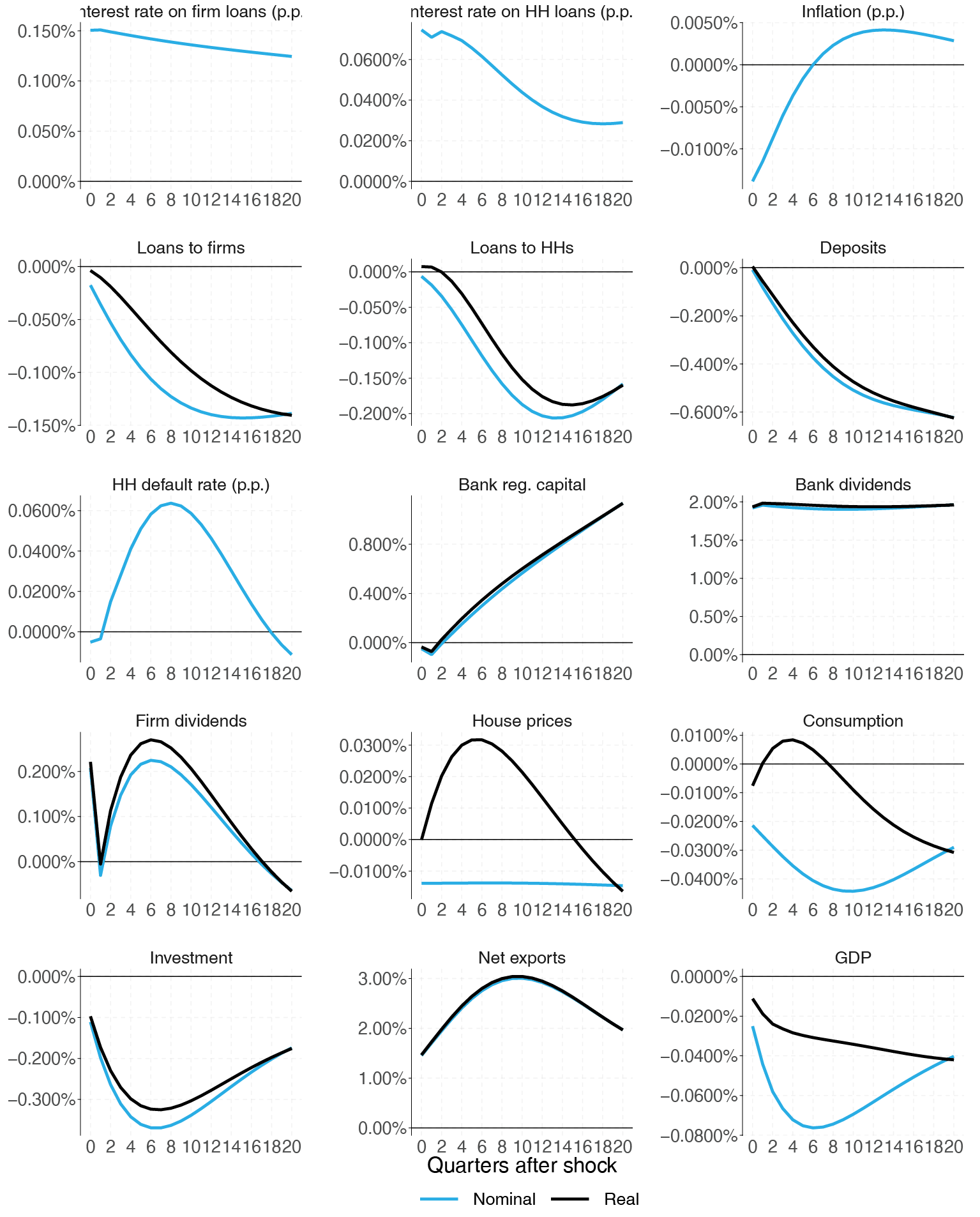
Figure 4. Responses to an unexpected and permanent rise in bank capital requirement by 1 p.p.

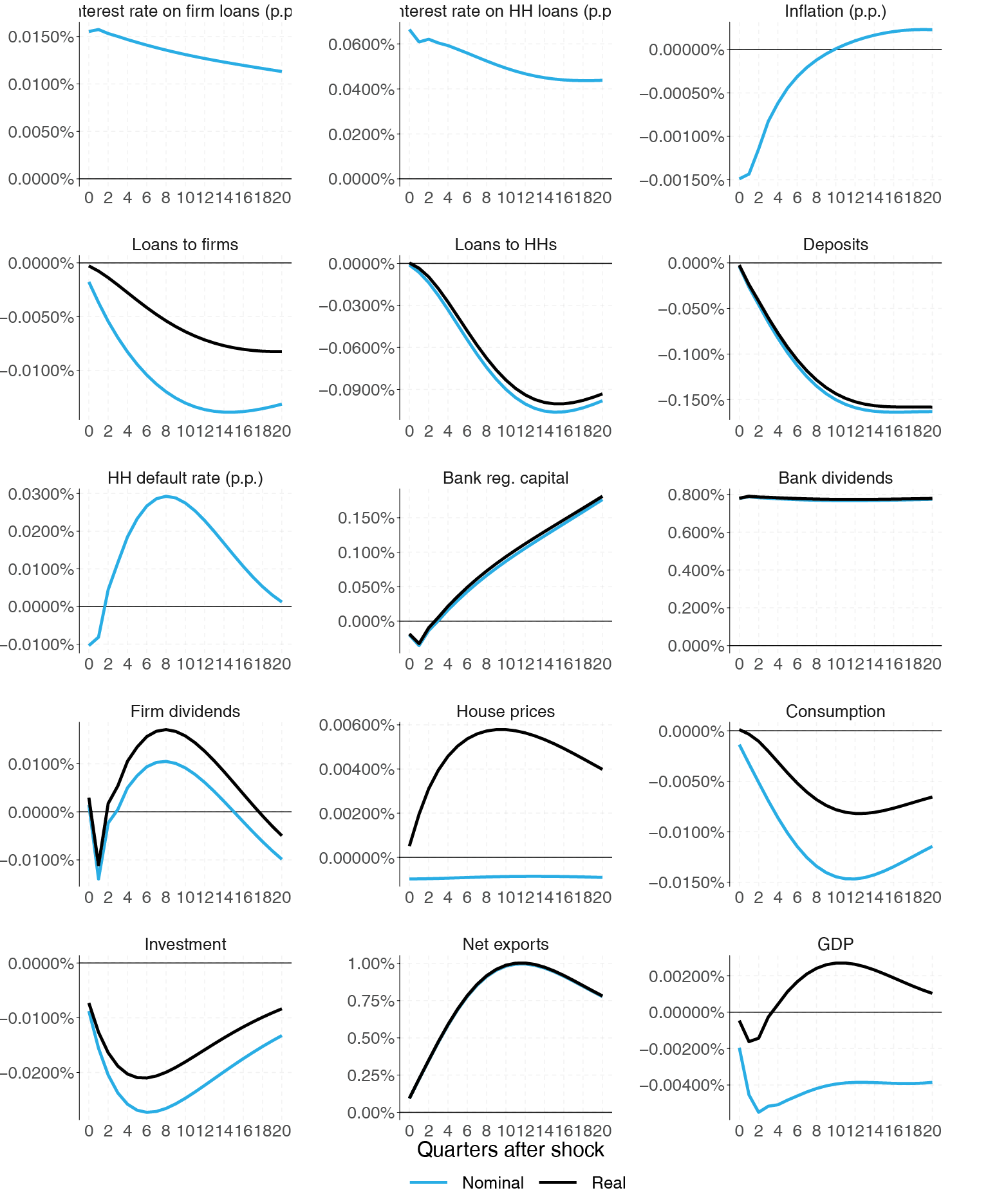
Figure 5. Responses to an unexpected and permanent rise in risk weight on mortgages by 5% (2.5 p.p. under baseline calibration).

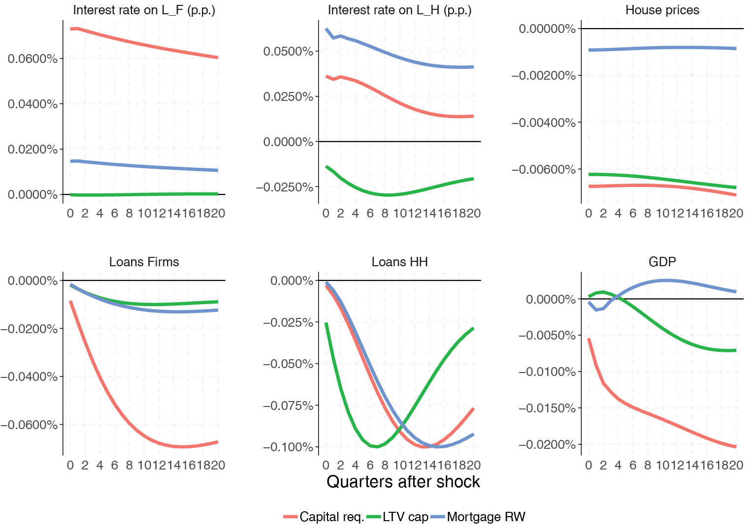
Figure 6. Main variable respones to equivalised three prudential policy tightenings: capital requirements, cap on LTV ratio and mortgage risk weight.

B. Alternative asset seizure

Here we describe the alternative first order conditions for impatient household and bank, when the bank is able to recover the whole amount defaulted. Under this setting asset seizure at time t is:

After plugging this into the impatient household’s budget constraint and solving the optimisation problem, the first-order conditions (11)-(13) respectively become:

Using this alternative asset seizure setting, the bank’s profit equation (18) becomes:

The first-order (mortgage supply) condition (26) is now:

C. Equation list

Here we state all equations of the baseline model.

D. Steady state

In the the steady state price and investment adjustment costs, as well as their respective partial derivatives, are equal to zero, and total factor productivity A is normalised to unity. Analytical derivation of the steady state is non-trivial because in the full model the interest rates on mortgages r^H depend on household default rate χ^H and vice versa. This creates a simultaneity issue that is hard to tackle algebraically. Hence, we do steady state derivation and calibration of the default rate simultaneously. First off, we assume a given quarterly default rate χ^H = 0.0125. Secondly, we recursively derive steady state expressions for model variables. Lastly, we choose a value of ψ_D so that the χ^H is consistent with annual default rate of 5%.

After finding the expressions for nominal value of mortgages, we calibrate ψ_D so that it is consistent with the target share of defaults χ^H:

Utilising the expressions for ratios above, we can obtain the steady state expressions for the following variables: F K W, L_F, F, K, W, P^H, DH, and π^B, Π^B. We can use these to obtain the rest of the variables.