Ekonomika ISSN 1392-1258 eISSN 2424-6166

2022, vol. 101(1), pp. 6–19 DOI: https://doi.org/10.15388/Ekon.2022.101.1.1

Determinants of Bilateral Trade Balance Between Georgia and China

Azer Dilanchiev
Department of Economics, Faculty of Business and Technologies,
International Black Sea University, IBSU, Tbilisi, Georgia
Email: adilanchiev@ibsu.edu.ge

Tengiz Taktakishvili
Faculty of Business and Technology, Georgian National University SEU, Tbilisi, Georgia
Email: t.taktakishvili@seu.edu.ge

Abstract. This paper aims to empirically examine the drivers of the bilateral balance of the trade model for the Georgian-Chinese economy from 2000 to 2020 and the influence of the Georgia-China free trade agreement on the Georgian-Chinese balance of trade. The Error Correction Model (ECM) of the ARDL was used to see if the balance of trade and its predictors have a long-term relationship. One of the ARDL’s defining properties is that it may be utilized in circumstances when there is minimal data, regardless of the level of variable integration. According to the findings, a perceived effective exchange rate has a statistically significant positive impact on the balance of trade in the long run and a statistically significant negative impact on the balance of trade in the short run. The output is shaped to favor the presence of the elasticity attitude’s J-Curve impact. The study also found that the comparative supply of money (MS) and GDP have only a minor impact on the trade balance in the medium and long run. The sponging and monetary methods are ineffective in characterizing the bilateral trade deficit between Georgia and China.
Keywords: ARDL, J-Curve, Error Correction Model (ECM), Balance of Trade, Real Effective Exchange Rate, Georgia, China.

_________

Received: 09/01/2022. Revised: 12/02/2022. Accepted: 12/02/2022
Copyright © 2022 Azer Dilanchiev, Tengiz Taktakishvili. Published by Vilnius University Press
This is an Open Access article distributed under the terms of the Creative Commons Attribution License, which permits unrestricted use, distribution, and reproduction in any medium, provided the original author and source are credited.

1. Introduction

Immediately upon gaining independence, Georgia attempted to reorganize its trade so that to establish domestic and international industries to boost the economy and encourage growth. In order to do so, it entered into several agreements with other countries, particularly those with stronger economies (Potjomkina, 2021). Georgia and China signed a free trade agreement in May 2017 that took effect in 2018. Georgia is one of the first countries to sign a free trade agreement with the People’s Republic of China. By establishing a free trade zone, the agreement lays the groundwork for increasing bilateral economic contacts between Georgia and China, including customs taxes, anti-dumping, and anti-monopoly measures. All of the benefits listed above can be applied immediately to the FTA with China (Lopatina, 2018).

According to World Trade Statistical Review 2020, the EU and China have a combined population of roughly 2 billion people and a market worth 32 trillion dollars, meaning that Georgia’s export-oriented industries may benefit from economies of scale (https://www.wto.org/english/res_e/statis_e/wts2020_e/wts2020_e.pdf). Thanks to a signed Free Trade Agreement (FTA) with China, Georgia has tremendous potential to attract FDI, technological advancements, and technical skills. It is worth mentioning that only seven countries have bilateral free trade agreements with both the EU and China. It allows Georgia to attract capital from foreign nations to export to the EU and capital from China to export to the EU.

This following research aims to analyze the drivers of the balance of trade for the Georgia-China economy and the impact of the free trade agreement of Georgia with China on the Georgia-China trade balance.

The free trade agreement can enhance Georgia’s economic growth, create jobs, and provide large and small enterprises with opportunities to profit from increased trade and investments. The free trade agreement can promote access to a greater range of competitively priced goods and services, new technologies, and creative practices for Georgian businesses and consumers. Free trade with China will also help China gain a foothold in the European Union market.

This agreement will potentially contribute to the development of trade relations between the two countries and increase its level. The Georgia-China Free Trade Agreement will help create favorable conditions for production in the private sector, which means bringing Georgian products to a market of 1.4 billion which is characterized by rapidly growing purchasing power. Georgia’s export is expected to grow significantly in the following years.

Georgia is a small, open economy country, while China’s exports have been steadily increasing for the past few years. Finalizing the free trade agreement with such a huge economy offers vast potential so that Georgia can become the most convenient, comfortable, and appealing platform for trading between large economies. Leading ranks in Doing Business, lower taxes, minimum administrative barriers and free trade with the European Union makes Georgia an interesting country for Chinese investors who can manufacture there and sell products to the EU countries. Chinese investments can be accompanied by an injection of new industrial technology knowledge. It should help with the modernization and recovery of Georgia’s export structure, which might serve as the foundation for developing a high purchasing power market in the EU.

The increasing trade volume between China and Georgia is one indicator of the unrevealed future potential. In Figure 1, data regarding Georgia’s export to China is given, and as it is evident that the importance of China as one of Georgia’s main trading partners has been dramatically increasing.

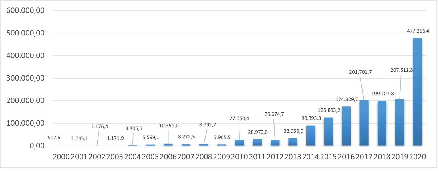
Figure 1. Georgia’s export to China, 2000–2020 (1,000s of USD)

Source: National Statistics Office of Georgia (https://www.geostat.ge/en/modules/categories/637/export)

Georgia has a positive trade balance with China, but, at the same time, Georgia’s import from China shows tremendous growth as well; see Figure 2.

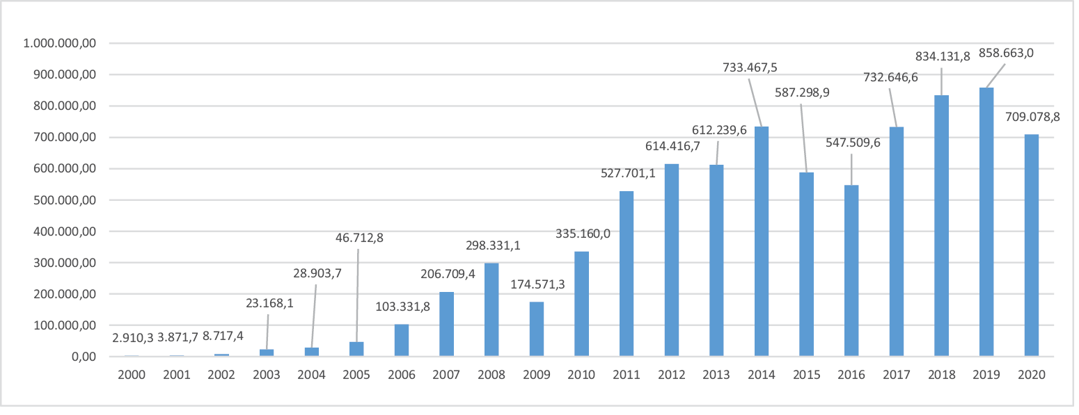
Figure 2. Georgia’s import from China, 2000–2020 (1,000s of USD)

Source: National Statistics Office of Georgia (https://www.geostat.ge/en/modules/categories/638/import)

The purpose of this article is to empirically assess the drivers of the bilateral balance of the trade model for the Georgia-China economy from 2000 to 2020 by using monthly data and the impact of the Georgia-China free trade agreement on the Georgia-China balance of trade.

In the literature, the Elasticities, Absorption, and Monetary approaches are used to explain the differences in trade balance deficits across countries. Each of these methods is based on different factors. Depreciation is used in the Elasticities approach to improve the trade balance. On the other hand, the Absorption method is based on the impact of revenue and price levels on the trade balance, while the Monetary approach assumes that monetary factors have an impact on the trade balance.

The paper discusses various studies that apply the ARDL model to evaluate the Georgia-China balance of trade from 2000 to 2020, while utilizing monthly data, in order to achieve the research goals of identifying the factors that tend to affect the Georgia-China balance of trade. The ARDL’s Error Correction Model (ECM) was used to determine if the balance of trade and its predictors have a stable long-run relationship. One of the ARDL’s distinguishing features is that it may be used in situations with limited data, regardless of the level of integration of the variables.

The ARDL model is employed to explicitly evaluate the bilateral trade balance between Georgia and China, which sets it apart from prior comparable studies. The research is divided into five sections. The first segment serves as an introduction, while the second section provides the theoretical framework and discusses the necessary studies. The study model is described in section three. The fourth section presents the empirical analysis, and the final section delivers the conclusion.

Researching this topic is valuable as it will be the first attempt to scientifically analyze economic effects of the above mentioned free trade agreement. It will be of interest for government officials as well as for business representatives. This agreement is one of the most important achievements of the last decade for the Georgia in terms of the deepening international trade relations; hence, research of its potential outcomes is of utmost importance.

2. Literature review

Elasticities, Absorption, and Monetary methods are utilized in the literature to explain variances in trade balance deficits between countries.

Iheanacho (2017) looked at the effects of trade liberalization on developing economies. The Autoregressive Distributed Lag (ARDL) bound test was used in this study. Two indicators of trade liberalization were utilized to create a trade openness index, while principal component analysis was employed to create a financial development index utilizing three measures of financial sector development. According to the findings, trade liberalization exerts detrimental long-term influence on Nigerian economic growth. Trade liberalization had a beneficial and large short-run impact on economic growth.

Bosnjak et al. (2018) examined the factors of the Croatian current account dynamics by using the monetary and Absorption approach. The paper’s fundamental hypothesis was that the Croatian current account could be explained in terms of the monetary and Absorption approach to the balance of payments. The study used the non-linear Auto-Regression Distributed Lag (NARDL) approach which considers the non-linear and asymmetric nature of the Croatian current account and its causes. Among the tested monetary variables, monetary aggregates M4 had the highest explanatory power. The paper’s major conclusions showed that fiscal policy measures and easing liquidity limitations for Croatian exporters must achieve external equilibrium.

Keho (2021a) showed that the trade balance is adversely correlated with domestic and foreign income but that real effective exchange rate depreciation improves the trade balance over time. The data, however, do not support the J-prediction curve of a short-run worsening of the trade balance. The trade balance was only responsive to foreign real income in the short run, but not to the domestic real income or the real exchange rate.

Adznan and Masih (2018) aimed to investigate the relationship between Malaysia’s exchange rate and its trade balance. By using more recent monthly time series data and relatively advanced methodologies, such as ARDL and NARDL, the study suggests a depreciation trade-off between the short and the long run and between exporting and importing industries. Policymakers could weaken the currency moderately to improve the trade balance, but they must efficiently manage the incurred costs.

Taşseven et al. (2019), by using quarterly data from 1998 to 2018, examined the factors of trade balance, such as Turkey’s gross domestic product, the GDP of some other nations (EU), real exchange rates, and oil prices. The cointegration model in use in Taşseven’s research is the ARDL (autoregressive distributed lag) bound testing approach. The findings of our study show that trade balance and its drivers have a cointegration connection. For Turkey, the long-term absorption technique has been verified. It was discovered that a rise in oil prices and a rise in the real exchange rate lower the trade imbalance significantly. By using the autoregressive distributed lag (ARDL) bound testing approach, a long-run relationship between Turkey’s gross domestic product, the gross domestic product of some other nations (EU), the real exchange rate, and oil prices is discovered. It was thus discovered that, in the long run, the gross domestic product of Turkey and the European Union countries has a positive and large impact on the trade balance, whereas the appreciation of the real exchange rate and oil prices has a significant negative impact on the trade balance. The findings are in line with the findings of other authors (Keho, 2021b). The author studied Ivory Coast’s non-linear link between the actual exchange rate movements and the trade balance. This work used multiple threshold non-linear ARDL modelling to evaluate possible signs and size-dependence in the reaction of the trade balance to the exchange rate. The cointegration test revealed that the real exchange rate, the gross domestic income, and the trade balance have a long-run relationship. The trade balance had a negative relationship with the gross domestic income, thereby indicating that increased domestic income decreases the trade balance. As a result, both in the short and in the long term, economic growth plays a vital role in lowering the trade deficit in Ivory Coast.

Waliullah et al. (2010), while discussing Pakistan’s economy, attempted to investigate the short and long-run link among the trade balance, the income, the money supply, and the real exchange rate. The model includes income and money variables to investigate the monetary and absorption approaches to the balance of payments, while the actual exchange rate is utilized to assess the traditional method of elasticities. The results revealed that the exchange rate depreciation is positively connected to the trade balance in the long and in the short run, which is consistent with the Marshall Lerner condition. The findings showed that the money supply and the income significantly shape the trade balance’s behavior. Although the exchange rate regime can help improve the trade balance, it has less impact than GDP and monetary policy. The study is in line with the findings of Duasa (2007). In the context of Malaysia, the author investigated the short- and long-run links between the trade balance, the real exchange rates, the income, and the money supply. The inclusion of the income and money variables in the study was intended to investigate the monetary and Absorption approaches to the balance of payments, in addition to the traditional elasticity approach based on exchange rates. The author analyzed whether a long-run equilibrium relationship between the trade balance and the determinants using the bound testing technique to cointegration and error correction models can be established inside an autoregressive distributed lag (ARDL) framework. By using the ARDL method, the study uncovered evidence of a long-run relationship between the trade balance and the income and money supply variables, but not between the trade balance and the actual exchange rate.

Ahad (2017) examined the relationship among the financial development, the trade balance, the exchange rate, and the inflation. The author used augmented Dickey-Fuller (ADF), Phillips-Perron, and breakpoint unit root tests to test the unit root attributes of variables. The autoregressive distributive lag (ARDL) method was used. The ARDL findings revealed the links among the long-term financial development, the trade balance, the exchange rate, and the inflation.

Labibah et al. (2021) aimed to look at the long-term and the short-term effects of inflation, exchange rates, and foreign economic growth on Indonesian exports. The Auto-Regressive Distributed Lag (ARDL) model was employed. According to the study’s findings, inflation and economic growth in China and Japan have a favorable and considerable effect on Indonesian exports. Furthermore, the short-term impact of the US exchange rate and economic growth on Indonesian exports is significant.

Karsten (2016) studied the short- and long-term link between the real effective exchange rate (REER) and the trade balance of 12 Eurozone countries. Panel data were employed, and each country was examined separately. The authors studied whether the depreciation of the euro and other drivers impact the trade balance by using the error correction form’s autoregressive distributed lag (ARDL) model. The study did not detect a significant short-term link between the two variables, while REER and the trade balance had a minor positive association in the long run, which correlates to a negative effect of depreciation on the trade balance. It is in direct opposition to the conventional macroeconomic theory.

The empirical findings of the study of Ditta et al. (2020) on the determinants of Finland’s trade balance showed that the real effective exchange rate, urbanization, and inflation have a significant but negative impact on Finland’s trade balance in both the short and the long run, while GDP per capita and unemployment have a significant but positive impact. The absence of any structural break in the model is confirmed by the plots of recursive estimates on both CUSUM and CUSUM square.

Widiyono et al. (2021) showed that the exchange rate is one of the most critical factors determining whether the balance is surplus or deficit. Indonesia’s trade balance is heavily influenced by China, as China is Indonesia’s major trading partner. According to this study, the Indonesia-China real exchange rate has a substantial and positive effect on the balance at lag one in the near run but has considerable and adverse effects on the balance in the long term. In the short run, the Indonesia-China real exchange rate has a considerable positive effect on the Indonesia-China balance of trade at lag one, but, in the long run, the exchange rate has a significant negative effect on the balance.

Yeshineh (2016) studied the short and long-run correlations of Ethiopia’s trade balance with some explanatory factors, such as the income, the money supply, the real exchange rate, the budget balance, and the foreign income being investigated in this article. The bound testing approach of cointegration and the error correction model, created inside the autoregressive distributed lag (ARDL) model framework, is applied to the annual data from 1970/71 to 2010/11 to determine whether there is a long-run link between the trade balance and its drivers. The study’s main finding is that the trade balance and its determinants have a consistent cointegration relationship (the real exchange rate, the income, the money supply budget balance, and the foreign income).

3. Model specification

The fundamental goal of this study is to assess the impact of the comparative GDP, the comparable real exchange rate, and the relative supply of money on the trade balance between Georgia and China. This study updates the strategy (Duasa, 2007; Kyereme, 2002) that utilizes the three approaches (Elasticities, Absorption, and Financial) to uncover the reasons for the balance of trade. We include a dummy variable to identify the impact of the Georgia-China free trade agreement on the balance of trade. The modified model may be represented as follows:

LBT = c + LGDP + LREER + LMS + DV + u (1)

LBT is the log of the balance of trade between Georgia and China. c is the constant that does not rely on the changes of the independent variables. LGDP is the log of the gross domestic product of Georgia compared to that of China. LREER is Georgian Lari’s log relative to Chinese Yuan’s actual effective exchange rate. LMS is the log of the relative money supply in Georgia compared to China. DV stands for a Dummy variable equal to 0 for the years when the free trade agreement between Georgia and China was not active and 1 when active. U is the error term.

In terms of approach, the study follows the concept created by Pesaran and Shin (1999; 1995) and expanded by Pesaran et al. (2001) by utilizing the Autoregressive Distribution Lag (ARDL) model to measure the long-run association between the mediator variable variables. This new model has various benefits, thereby making it superior to other models in predicting the long-term cointegration relationship. One of its primary advantages is that it can be utilized in small samples, independently of the degree of integration of the variables. The drivers of the Georgia-China trade balance shall be calculated with a model evaluating the long-term connection between the model’s variables. In order to examine the presence of such a long-run relationship, the bound cointegration test shall be utilized.

In order to perform the bound test approach for Equation (1), the Error Correction version of the ARDL model is supplied correspondingly by the Unrestricted Error correction representation (UECM) of the ARDL as follows:

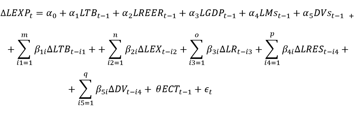(2)

Where Δ is the first difference operator and m, n, o, p, q are optimal lags in the model, α and β are coefficients, θ is the coefficient of the error correction term (ECT) estimating the speed of adjustment to equilibrium (θ should be negative and between 0 and -1), and εt is a white noise disturbance error term.

Before the application of the ARDL approach, the stationarity of the variables was evaluated to guarantee that all elements are stationary on I (0), I (1), and that no factors are integrating of order (2) or higher. The next stage, the long-term connection using the ARDL technique, was applied, which requires two phases: the first objective is to test the long-run connection across all factors in the model by utilizing the bound cointegration test based on the critical value. In order to identify a long-run connection, it is recommended to move to the second stage evaluating the model’s short- and long-run coefficients. Various diagnostic procedures ought to be implemented to verify the reliability of the proposed model, and various residual tests were implemented, beginning with the white test and ARCH tests for heteroscedasticity, the Jarque-Bera test for the Normality of data, the Breusch-Godfrey LM test for serial correlation, and Ramsey’s RESET to check the structural model measurement errors. Also, CUSUM and CUSUMQ examine the robustness of the long-run characteristics.

4. Empirical findings

The results of the Augmented Dickey-Fuller (ADF) and Phillips-Perron (PP) unit root analyses based on the Schwarz information criterion (SIC) are given in Table 1.

Based on Table 1, all the variables are non-stationary at a level except the logarithm of the balance of trade (LBT) which is stationary at level (0). All the variables become stationary with the first difference (I). The unit test result indicates a combination of stationary variables at level (0) and the first difference (I). The ARDL method has the benefit of generating asymptotically normal estimates of the long-run coefficients, regardless of whether the underlying regressors are I(1), I(0), or a combination of both (Pesaran, 1998). According to Menegaki (2019), each variable must be I(0) or I(1) or a combination to satisfy the limits test assumption of the ARDL models. It was also determined by Dilanchiev and Taktakishvili (2021) that the ARDL bound test approach is optimal for the analysis’ estimate procedure due to the combination of stationary variables at level I(0) and the first difference I(1).

Table 1. Unit root test for stationarity

ADF			PP
Variables	Level	First difference	Level	First difference
LTB	-3.7205**	-16.711***	-7.3101***	-22.6331***
LREER	-2.0336	-13.563***	-1.8771	-13.4126***
LMS	-2.1071	-18.207***	-1.9307	-18.9655***
LGDP	-1.9317	-16.0021***	-1.9670	-16.0101***
1%	-3.456408	-3.456514	-3.456302	-3.456408
5%	-2.872904	-2.872950	-2.872857	-2.872904
10%	-2.572900	-2.572925	-2.572875	-2.572900

Notes: *** Significant at 1%, ** Significant at 5%, * Significant at 1%

4.1. ARDL Outcomes

To assess the coefficient of the long-run relationships and the corresponding error correction model (ECM) through using the ARDL model, the sequence of distributed lag on the predictor variable was chosen by the Akaike information criterion (AIC) which designates an ARDL (2,4,0,2,0) for the measurement used in the model.

4.1.1. Co-integration Analysis (Bound Test)

For evaluating the long-run cointegration connection among the parameters, the bound test employed derived F-statistics from the statistical significance of lagged levels of the parameters applied to indicate the existence of cointegration. The outcome of the Wald test (F-statistics) is provided in Table 2.

Table 2. F statistics and bound test

Model	k	M	F statistics	Significance level	Lower bound	Upper bound
ARDL (2,4,0,2,0)	4	4	5.171285*	10%	2.2	3.09
				5%	2.56	3.49
				1%	3.29	4.37

Notes: M indicates maximum lags, k expresses explanatory variables, and * shows significance at 1%

Table 2 shows that the trade balance, the predictor variable, and the real GDP are cointegrated, with the F statistics derived in Table 2 being greater than the upper critical threshold statistically significant at less than 1% level. Because the presence of a cointegrated link is determined in this manner, the estimate of Autoregressive Distributed lag (ARDL) models started in addition to finding the long- and short-term correlations.

4.1.2. Short-run and long-run analysis

The assessment outcome of the long-run ARDL analysis is presented in Table 3 which gives the long-run coefficients. Table 3 contains the Measured Long Run Coefficient values applying the ARDL method.

Table 3. Estimated ARDL (2,4,0,2,0) Long-run model

Variable	Coefficient	t-Statistic
LEER	1.125790	4.106409***
LMS	1.753246	1.889200**
LGDP	-3.561316	-1.866327**
DV	-1.137968	-1.747233*
C	0.841663	0.466273

Notes: *** Significant at 1%, ** Significant at 5%, * Significant at 10%

The component of REER is shown to be statistically significant at the 1 percent level, meaning that, in the long term, the relative exchange rate getting higher by 1 percent would increase the balance of trade deficit by 1.126 percent. In the short term (Table 4), the relative exchange rate has a significant influence on the balance of trade, as a 1 percent rise in the relative exchange rate would cause a reduction in the trade balance by 4.323 percent.

All the other variables proved statically unimportant in the short term. The coefficients of comparative supply of money LMS and comparative LGDP were modestly significant contrasted with the real exchange rate REER, at less than 10 percent significance level. Notwithstanding the indications of such coefficients, they partially overlap with the conceptual and the scientific implication of permeation and budgetary concepts, which implies that the rate of exchange of the Georgian Lari against the Chinese Yuan is the primary factor in the explanation of the conduct of the balance of trade between Georgia and China in the short and long term.   The findings follow the economic theory, as the rising exchange rate of the Georgian Lari, in the long run, would then enhance the efficacy of China’s goods to the Georgian commodities in the Georgia and China markets. It consequently can lead to a reduction of Georgian products in the China market (attributable to an increase in the price of the Georgian goods) and substitute the Chinese commodities instead of Georgian imports. Furthermore, replacing Chinese imports instead of domestic goods in the Georgian economy can lead to low prices.

In the short run, a rise in the currency value of the Georgian Lari against the Chinese Yuan might result in a rise of consumption of Chinese goods and a decline in the currency value of the Chinese Yuan, resulting in an rise in the prices of the bill for the China imports from Georgia and a fall in the cost of the fee for Georgian imports from China, thereby resulting in redistribution.

The estimated outcome also indicates that the influence of the dummy variable (the trade treaty between Georgia and China) is statistically insignificant on the balance of trade in the long term. It means that the trade treaty cannot influence the balance of trade between these nations. Furthermore, this positive link (non-significant) is compatible with the theoretical framework in the liberalization of the world trade. The outcome also validates the state’s policy which has cancelled the treaty’s regulations. The Error Correction term (ECT) identifies the directions and the pace of the correction in the equation owing to any short-term disequilibrium by assessing the value and the statistical evidence of ECT. The presence of ECT with a negative sign and a statistically significant value implies that an integrated long-run connection may be established among the factors in the model, hence rectifying the short-run departure of the balance of trade from the long-term equilibrium demands.

Cointeq = LTB − (0.841663C+1.125790LREER + 1.753246LMS − 3.561316LGDP --1.137968DV)

Table 4. Estimated ARDL (2, 4, 0, 2, 0) Short-run model

Variable	Coefficient	t-Statistic
ECT (-1)*	-0.353597	-5.549168***
D(LTB(-1))	-0.330225	-5.549168***
D(LREER)	-4.323081	2.005861***
D(LREER(-1))	-1.777109	2.268697***
D(LREER(-2))	5.313655	-0.783317
D(LREER(-3))	-1.777109	2.268697***
D(LGDP)	-3.498070	-2.029596***
D(LGDP(-1))	0.274726	1.925964*

Notes: *** Significant at 1%, ** Significant at 5%, * Significant at 1%

4.1.3 Diagnosis and Stability Tests

ECT, following (Banerjee et al., 1998), denotes the speed modification required to reestablish equilibrium in the dynamic model. ECT is a statically significant factor with a negative sign demonstrating how rapidly parameters converge to equilibrium. The relatively substantial ECT adds to the evidence of a long-term link that is robust.

The ARDL approach satisfies the usual diagnostic tests, as indicated in Table 5. The normality test was performed with Jarque-Bera Test, and it was found that residual variables were normally distributed 0.514288. Neither serial correlation was identified through LM Test with a likelihood of 0.128128 nor heteroscedasticity via a Breusch-Pagan-Godfrey test of 0.615254. The Ramsey RESET Test implies that the model is tabling, and there is no issue with identification 0.443544The CUSUM Statistics and CUSUM Square Stability Test is within the 5% significance level boundaries, thus indicating that the applied ARDL model is stable and robust.

Table 5. Test Statistics

X2BG 0.128128 (0.6036)	X2JB 0.514288 (0.8124)
X2BPG 0.615254 (0.2302)	X2 Ramsey 0.443544 (0.6143)

Notes: X2BG is the Breusch-Godfrey Serial Correlation LM Test employed to verify serial correlation, X2BPG is the Breusch-Pagan-Godfrey test applied to verify heteroscedasticity, X2JB is the Jarque-Bera test applied to verify the Normality, and X2Ramsey is applied to verify if the model is properly defined.

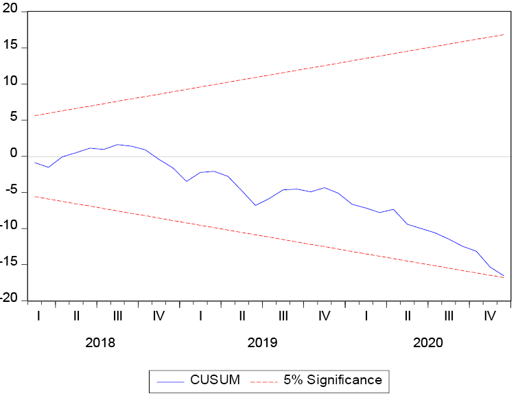
Figure 3. Plot of CUSUM Statistics for Stability Test

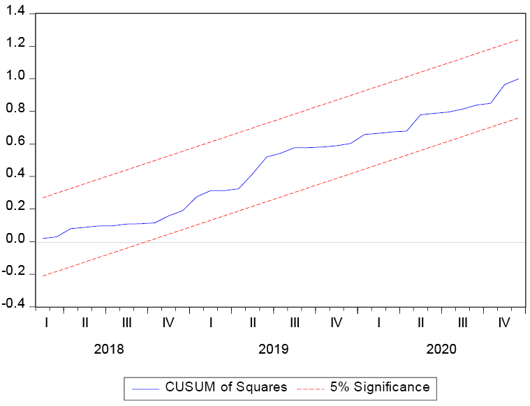
Figure 4. Plot of CUSUM(Q) Statistics for Stability Test

5. Conclusion

This research intended to analyze the drivers of the bilateral trade balance model for the Georgia-China economy and the influence of the free trade treaty with China on the Georgia-China trade balance by employing empirical monthly data spanning across the period from January 2000 to December 2020. The research employed the Autoregressive Distribution Lag (ARDL) model to assess the long-term relationship between dependent and independent variables. We followed the developed model which applies the three techniques to find the factors of the balance of trade. The research outcome concluded that a perceived effective exchange rate exerts a statistically significant positive impact on the balance of trade in the long term and adverse influence on the balance of trade in the shorter term. The result follows a way that favors the presence of the J-Curve impact of the elasticity attitude. The study also demonstrated that the comparative supply of money (LMS) and LGDP has modest influence on the balance of trade in the short and in the long term, thereby implying that the sponging and monetary method is not appropriate for describing the bilateral balance of the trade imbalance between Georgia and China. The estimated finding suggests that the influence of the trade treaty between Georgia and China is minor on the balance of trade in the long term, which justifies the viewpoint of the state which has cancelled the activity on this treaty. The most significant policy inference to be derived from these empirical results is that the depreciation of Georgian Lari versus Chinese Yuan may be employed to effect an adjustment in the balance of trade of Georgia against China.

The implementation of the Free Trade Agreement will intensify trade between the two countries. As a result of the free trade agreement, Chinese households will be able to buy Georgian wine, mineral water, vegetables, and tea. Free trade with China is a new opportunity for Georgia to diversify its market and increase exports. In addition, entering the Chinese market is a significant incentive for companies to expand production and make additional investments. At the same time, against the background of strengthening economic relations between the two countries, Georgia will become even more attractive to Chinese investors.

Nevertheless, raising the comparative supply of money or decrease will not accomplish the intended purpose. Therefore, statistics from other nations (rather than one country) can be utilized to investigate the trade balance for the following research. Furthermore, instead of the overall export and import numbers as the totality, specific sector statistics figures could be employed to identify the drivers of the trade balance.

References

Adznan, S., & Masih, M. (2018, December 30). Exchange rate and trade balance linkage: Evidence from Malaysia based on ARDL and NARDL [MPRA Paper]. https://mpra.ub.uni-muenchen.de/91509/

Ahad, M. (2017). Impact of Financial Development on Trade Balance: An ARDL Cointegration and Causality Approach for Pakistan. Global Business Review, 18(5), 1199–1214. https://doi.org/10.1177/0972150917710152

Banerjee, A., Dolado, J., & Mestre, R. (1998). Error-correction Mechanism Tests for Cointegration in a Single-equation Framework. Journal of Time Series Analysis, 19(3), 267–283. https://doi.org/10.1111/1467-9892.00091

Bosnjak, M., Novak, I., & Krišto, A. (2018). Monetary and absorption approach to explain the Croatian current account *. Zbornik Radova Ekonomskog Fakulteta u Rijeci / Proceedings of Rijeka School of Economics, 36, 929–946. https://doi.org/10.18045/zbefri.2018.2.929

Dilanchiev, A., & Taktakishvili, T. (2021). Currency Depreciation Nexus Country’s Export: Evidence from Georgia. Universal Journal of Accounting and Finance, 9(5), 1116–1124. https://doi.org/10.13189/ujaf.2021.090521

Ditta, A., Asim, H., & Rehman, H. U. (2020). An Econometric Analysis of Exigent Determinants of Trade Balance in Finland: An Autoregressive Distributed Lag (ARDL) Approach. Review of Applied Management and Social Sciences, 3(3), 347–360. https://doi.org/10.47067/ramss.v3i3.69

Duasa, J. (2007). Determinants of Malaysian trade balance: An ARDL bound testing approach. Global Economic Review, 36(1), 89–102.

Iheanacho, E. (2017). ARDL Approach to Trade Libralisation and Economic Growth in the Developing Country: Evidence from Nigeria. African Research Review, 11(2), 138–159. https://doi.org/10.4314/afrrev.v11i2.11

Karsten, V. (2016). Short and long run effects of exchange rate movements on the trade balance: A Eurozone perspective.

Keho, Y. (2021a). Determinants of Trade Balance in West African Economic and Monetary Union (WAEMU): Evidence from Heterogeneous Panel Analysis. Cogent Economics & Finance, 9(1), 1970870.

Keho, Y. (2021b). Effects of Real Exchange Rate on Trade Balance in Cote d’Ivoire: Evidence from Threshold Nonlinear ARDL Model. Theoretical Economics Letters, 11(3), 507–521. https://doi.org/10.4236/tel.2021.113034

Kyereme, S. S. (2002). Determinants of United States’ trade balance with Australia. Applied Economics, 34(10), 1241–1250. https://doi.org/10.1080/0003684011-0094437

Labibah, S., Jamal, A., & Dawood, T. C. (2021). Indonesian Export Analysis: Autoregressive Distributed Lag (ARDL) Model Approach. Journal of Economics, Business, & Accountancy Ventura, 23(3), 320–328.

Lopatina, I. (2018). Georgia: Georgia signs free trade agreement with China. International Tax Review. https://www.internationaltaxreview.com/article/b1f7n3d4sy1h2f/georgia-georgia-signs-free-trade-agreement-with-china

Menegaki, A. N. (2019). The ARDL Method in the Energy-Growth Nexus Field; Best Implementation Strategies. Economies, 7(4), 105. https://doi.org/10.3390/economies7040105

Pesaran, M. H. (1998). An Autoregressive Distributed-Lag Modelling Approach to Cointegration Analysis. In S. Strøm (Ed.), Econometrics and Economic Theory in the 20th Century: The Ragnar Frisch Centennial Symposium (pp. 371–413). Cambridge University Press. https://doi.org/10.1017/CCOL0521633230.011

Pesaran, M. H., & Shin, Y. (1995). An autoregressive distributed lag modelling approach to cointegration analysis.

Pesaran, M. H., Shin, Y., & Smith, R. J. (2001). Bounds testing approaches to the analysis of level relationships. Journal of Applied Econometrics, 16(3), 289–326. https://doi.org/10.1002/jae.616

Pesaran, M. H., Shin, Y., & Smith, R. P. (1999). Pooled mean group estimation of dynamic heterogeneous panels. Journal of the American Statistical Association, 94(446), 621–634.

Potjomkina, D. (2021). Inclusion in EU-Georgia Trade Relations: A Critical Institutionalist Analysis of the Georgian Domestic Advisory Group. European Foreign Affairs Review, 26(3).https://kluwerlawonline.com/journalarticle/European+Foreign+Affairs+Review/26.3/EERR2021035

Taşseven, Ö., Saracel, N., & Yılmaz, N. (2019). Determinants of trade balance for Turkey: ARDL based bounds testing approach.

Waliullah, W., Khan Kakar, M., Kakar, R., & Khan, W. (2010). The Determinants of Pakistan’s Trade Balance:An ARDL Cointegration Approach. THE LAHORE JOURNAL OF ECONOMICS, 15(1), 1–26. https://doi.org/10.35536/lje.2010.v15.i1.a1

Widiyono, Y., Ismail, M., & Saputra, P. M. A. (2021). THE EFFECT OF EXCHANGE RATE ON INDONESIA-CHINA BALANCE OF TRADE.

Yeshineh, A. (2016). Determinants of Trade Balance in Ethiopia: An ARDL Cointegration Analysis. https://doi.org/10.2139/ssrn.2854178