Ekonomika ISSN 1392-1258 eISSN 2424-6166

2022, vol. 101(1), pp. 125–141 DOI: https://doi.org/10.15388/Ekon.2022.101.1.7

Dynamics of Exchange Rate Fluctuations in Turkey: Evidence from Symmetric and Asymmetric Causality Analysis

Ali Çeli̇k
Istanbul Gelisim University, Turkey
Email: alcelik@gelisim.edu.tr
ORCID: https://orcid.org/0000-0003-3794-7786

Abstract. This study examines the factors affecting exchange rate fluctuations in Turkey by employing the quarterly data from 2008 to 2020. In this context, linear and nonlinear unit root tests were used to determine the stationarity levels of the variables. Then, symmetric and asymmetric causality analysis was preferred to ascertain the relationship between the variables. Symmetric causality analysis results indicated a causality relationship from the exchange rate to the long-term debt stock, from the credit default swap (CDS) to the exchange rate, and from the exchange rate to the uncertainty index. The asymmetric causality analysis showed a causality relationship from positive shocks in the short-term debt stock to negative shocks in the exchange rate. Also, it was proven that there exists a causality relationship from negative shocks in the short-term external debt stock to positive and negative shocks in the exchange rate. Another result demonstrated a causality relationship between positive shocks in the exchange rate to negative shocks in the long-term debt stock. In addition, it was found that negative shocks in net capital investment were the cause of negative shocks in the exchange rate, while it was determined that there was a causality relationship from positive shocks in the net reserves to positive shocks in the exchange rate. In conclusion, the asymmetric causality relationship from positive shocks in CDS to positive shocks in exchange rates was detected.
Keywords: Exchange Rate, Non-Linear Unit Root Test, Symmetric Causality Analysis, Asymmetric Causality Analysis

_________

Received: 28/01/2022. Revised: 04/03/2022. Accepted: 20/03/2022
Copyright © 2022 Ali Çelik. Published by Vilnius University Press
This is an Open Access article distributed under the terms of the Creative Commons Attribution License, which permits unrestricted use, distribution, and reproduction in any medium, provided the original author and source are credited.

1. Introduction

Worldwide, the exchange rate regime has been exposed to significant changes after the Bretton Woods system was ended. Therefore, the exchange rate regime fixed to gold has been completed, and the flexible exchange rate regime has begun. Besides, the transition to a floating (flexible rate) exchange rate regime opened the way for the movements of financial capital¹. The countries with fragile economic structures often faced extreme fluctuations, sharp ups and downs in exchange rates, together with the floating exchange rate regime. Especially after the 1990s, excessive financialization and the exchange rate regime has been playing an essential role in the exchange rate, banking, and financial crises, especially in late-capitalist countries, including Turkey. Despite such practices as the exchange rate adjustment and the liberalization of capital movements after 1980, the Turkish economy switched to the floating exchange rate regime after the 2001 crisis. Mainly, the market players determine the exchange rate in the floating exchange rate regime unless the dirty floating exchange rate regime is applied. Accordingly, the exchange rate is directly connected to the market initiative, so when the monetary authority does not control the exchange rate, it becomes problematic to restrain the excessive volatility of the exchange rates. It should be said that the sharp volatility of the exchange rates is associated with many factors, such as economic and political factors. In the literature, the increase or decrease in the exchange rates is differently defined according to the exchange rate regimes. For instance, in the floating exchange rate regime, the upsurge in the exchange rate implies depreciation, while the decrease in the exchange rate is expressed as appreciation (Hepaktan, 2009).

The main purpose of this study is to test the asymmetric and symmetric causality linkages between the factors affecting the fluctuations in the exchange rate after the 2008 global economic crisis in Turkey. In this context, the study seeks to (i) analyze the stationarity of variables by employing both linear and non-linear unit root tests, (ii) investigate the relationship between variables by employing symmetric causality analysis, and (iii) examine the relationship between variables by employing asymmetric causality analysis. For this purpose, the study is designed to consist of 6 sections. After the introduction part in Section 1, the literature review on the subject is included in Section 2. In Section 3, the study data and methodology are presented. The analysis findings are delivered in Section 4, while the results of the study are outlined in Section 5. The discussion part constitutes Section 6.

2. Related Literature Review

It is argued that risk and uncertainty prevail as a natural consequence of a highly fragile economic structure that relies heavily on outside financial sources. It is clear that the macroeconomic indicators which form the basis of the country’s economic dynamics may follow a fluctuating course under the dominance of these conditions. The exchange rate indicator is also directly affected by this structure. It is known that exchange rate volatility is a substantial element of the competitiveness of economies and has a central function in open economies, especially in those countries where the dependency ratio of exports to imports is high. For this reason, there are many studies on the subject. Some of the studies carried out in this context are as follows. Şimşek (2014) estimated the long-term determinants of the real exchange rate in Turkey. In addition, the Autoregressive Distributed Lag (ARDL) bounds test approach was used for this analysis. He revealed that the money supply (M2), the net foreign capital inflow, the foreign trade balance, and the terms of trade affect the real exchange rate. İlgün et al. (2004) investigated the impact of budget deficits on the real exchange rate in the Turkish economy by applying the ARDL bounds test. That analysis was using monthly data covering the period 1994:Jan–2012:Dec. The study indicated that the inflation rate and budget deficits cause fluctuations in the real exchange rate. Şit and Karadağ (2019) examined any relationship between the exchange rate and the effect of the foreign trade deficit, money supply (M2), the current account deficit, the interest rate, the foreign exchange reserve, and the consumer price index on the exchange rate by employing the ARDL bound test. According to the analysis results, all variables positively impacted the exchange rate except for the interest rate variable. Unlike previous studies, Şarkaya (2019) examined the factors affecting the real effective exchange rate by using heterogeneous panel data analysis specific to BRICS-T. The results determined that positive developments in reserve assets are reflected similarly to the real effective exchange rate. At the same time, different findings are reached across each country, while changes in the monetary base, the consumer price index, and oil prices have positive results for some countries and negative results for some other countries as well. Akduğan (2020) analyzed the relationships between the public debt and the exchange rate in Turkey by using a time series span from 2002 to 2019. This study used Johansen cointegration and VEC analysis. It was argued that the rise in the country’s debt stock, in general, harmed the real exchange rate, especially if foreign currency borrowing was made, while the changes in the real exchange rate affected the domestic debt stock and the total debt stock was in Turkish Lira. Tatar and Erdogan (2020) examined the exchange rate and foreign debt relationship by considering a wider historical process covering the years 1970 to 2018 in their study for Turkey. As a result of the VAR and Granger causality analysis, it was determined that the effect of foreign debt on the exchange rate was stronger than the effect of the exchange rate on the external debt. Makhdom (2021) investigated the relationship between macroeconomic indicators and the exchange rate by time series analysis (for the period 2005:Jan–2019:Oct) in Turkey. It was found that the selected variables had a long-term cointegration relationship. While it was evident that the exchange rate had a positive relationship between the interest and inflation, in the long run, it was determined that the dependent variable in question had an opposite relationship with the foreign trade balance, money supply, and unemployment. In addition, it was proven that there was only negative relationship between the exchange rate and the foreign trade balance in the short run. At the same time, there was a positive relationship in terms of other variables. Some examples from the national literature on the factors determining the exchange rate were examined, and then the international literature dealing with this issue was generalized upon. Suthar (2008) investigated the variables affecting the exchange rate in India. This study used monthly data between April 1996 and June 2007. Unlike other variables discussed in the literature review, the short and long-term interest rates and the interest yield differences, and foreign exchange reserves significantly influenced the Indian Rupee’s value compared to the foreign currency. Carrera and Restout (2008) investigated the long-term behavior of the real exchange rates of nine Latin American countries while covering the years 1970 to 2006 by using panel data analysis. As a result of that study, the Balassa-Samuelson effect, public expenditures, the terms of trade, the degree of openness, foreign capital flows, and the actual nominal exchange rate were detected as long-term determinants of the real exchange rate. Saeed et al. (2012) examined the effect of factors on the real exchange rate for Pakistan by using monthly data from January 1982 to April 2010. They found that the Pakistan Rupee against the US dollar was affected by the debt stock, the money supply, and the Foreign Exchange reserves. These results were obtained by applying the ARDL bounds test or the Error Correctional Model. Oriavwote and Oyovwi (2012) analyzed the impact of factors on the real effective exchange rate for Nigeria between 1970 and 2010. The study’s analysis was based on the Johansen cointegration test and the error correction model. Johansen’s cointegration analysis results indicated a long-term relationship between the examined variables. They proved that the real effective exchange rate was deeply affected by the nominal exchange rate, the capital inflow, and the inflation rate. Many studies explain the determinants of exchange rate fluctuations for different countries by time series and panel data analysis. In this context, Chowdhury and Hossain (2015), Benazic and Skabic (2016), Raza and Afshan (2017), Hassan and Dantama (2017) and Phuc and Duc (2021) investigated the factors affecting the exchange rate in Bangladesh, Croatia, Pakistan, Nigeria, and the Asia-Pacific region, respectively, while Elfaki (2018), Barbosa et al. (2018), Mungule (2020), He et al. (2021) and Raksong and Sombatthira (2021) examined the determinants of the exchange rate for Sudan, the developing and emerging countries, Zambia, China, and the emerging ASEAN counties, respectively.

3. Study Data and Methodology

This section examines the study data and the methodological dimension of the econometric tests. It starts with the study data, and then the econometric method part is discussed.

3.1. Study data

This study employs quarterly data from 2008Q1 to 2020Q4. Secondary data obtained from the Electronic Data Distribution System organized by the Central Bank of the Republic of Turkey (EVDS) (www.investing.com) and the International Money Fund (IMF) is used. Table 1 presents the characteristics of the study data.

Table 1. Variable’s specification

Variables	Abridgment	Data	Sources
Exchange Rate	LNER	Natural Logarithm	EVDS
Short Term Debt	LNSTD	Natural Logarithm	EVDS
Long Term Debt	LNUTD	Natural Logarithm	EVDS
Credit Default Swap (CDS)	LNCDS	Natural Logarithm	www.investing.com
Uncertainty Index	LNUNC	Natural Logarithm	IMF
Net Reserve	NETRES	Rate	EVDS
Net Capital Investment	NETCAP	Rate	EVDS
Real Interest Rate	RIR	Rate	EVDS

3.2. Methodology

This subtitle examines the theoretical background of the unit root and causality tests. First, the necessary information should be given about the methodological origin of the linear, the non-linear, and the non-linear with Fourier function unit root test methods used in this study.

3.2.1. Linear and Nonlinear Unit Root Tests

The Augmented Dickey-Fuller (1979, 1981) and Phillips Perron (PP) unit root tests are the most preferred linear unit root tests. In this study, Table 2 and Table 3 indicate the Augmented Dickey-Fuller (ADF) and PP unit root test results, respectively. Following that, we also evaluate the nonlinear test models as it is known that there is mostly no linear relationship between the variables. Therefore, after applying the ADF and PP unit tests, we focus on the nonlinear unit root test. We preferred the smooth transition autoregressive models (STAR) to estimate the nonlinear relationship between the variables. STAR gained popularity in modeling economic and financial data dynamics (Terasvirta, 1994). The exponential smooth transition autoregressive model (ESTAR) and the unit root tests are referred to in this section. The ESTAR process is formulated as follows (Kruse, 2011: 73-75):

Δy_t = αy_t–1 + θy_t–1 (1 – exp{–γ(y_t–1 – c)²}) + ε_t (1)

Under conditional ε_t~iid (0, σ²), ‘‘γ’’ defines the smoothing parameter, whenever γ approaches zero, the Linear AR (1) model emerges instead of the ESTAR model. In the model, c is described as a threshold value. Kapetanios et al. (2003) define the ESTAR model under the constraint (α=0) as follows:

Δy_t = θy_t–1 (1 – exp{–γ(y_t–1 – c)²}) + ε_t (2)

Where, if it is in the range of -2< θ<0 for the case of y_t–1=c, since it contains a unit root partially, although it is not locally stationary, the global stationarity condition is satisfied. Accordingly, under conditional constraint θ=0, the random walk process works well. Another assumption made by Kapetanios et al. (2003) is shown under the c=0 constraint:

Δy_t = θy_t–1 (1 – exp{–γ(y_t–1)²}) + ε_t (3)

Kruse (2011) considers the following non-stationary time series model to allow for the case where the indicator function (c) is not equal to zero (c≠0) within the exponential transition function:

Δy_t = θy_t–1 (1 – exp{–γ(y_t–1 – c)²}) + ε_t (4)

In the equation, Kapetanios et al. (2003), by using the first-order Taylor expansion, made the model take the following form:

Δy_t = β₁ y³_{t –1} + β₂ y²_{t –1} + β₃ y_t–1 + ε_t (5)

By following Kapetanios et al. (2003), Kruse (2011) accepts β₃=0 to increase the test power. After that, the latest model is as follows:

Δy_t = β₁ y³_{t –1} + β₂ y²_{t –1} + ε_t (6)

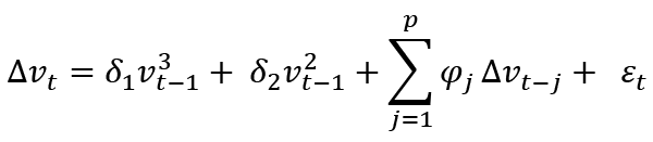
It is expressed in the equation as β₁=γθ and β₂=-2cγθ. The standard Wald test is not suitable for Kruse (2011) unit root testing. Thereby, MWald test proposed by Abadir and Distaso (2007) was used. The null hypothesis (H₀:h(θ) ≡ [h₁(θ) = h₂(θ)]' = [β₁β₂]' = [0,0]) demonstrates that the variables have a unit root, and the alternative hypothesis demonstrates (H₁:h₁(θ) < 0 or h₂(θ) ≠ 0)that the series are a stationary ESTAR process for this test. Kruse (2011) also calculated the test statistics in the same way as Kapetanios et al. (2003). That is, the test statistics are calculated for raw data (Case 1), demanded data (Case 2), and detrended data (Case 3). In addition, Sollis’s (2009) nonlinear unit root test is applied in this study. In this direction, Sollis’s (2009) test statistics can be calculated as follows:

(7)

When supposing k=0 in the following equation ,
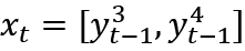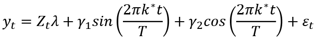
it follows that , m=2, R=2x2 matrix, , φ1 and φ2 are given LS estimator for and, , r = [0,0]' and is the LS estimate of . In addition, F_AE, F_AE,_μ, F_AE,_t denote the test statistics for testing H₀:φ₁=φ₂=0 for the zero mean, the non-zero mean and the deterministic trend cases, respectively (Sollis, 2009: 121). Güriş (2019) contributed to the econometrics literature by adding Fourier functions to the nonlinear unit root test model. This test examining structural breaks and nonlinearity provides a substantial opportunity. Güris’s (2019) test procedure² can be shown as follows:

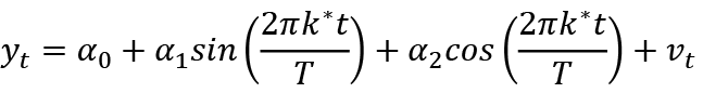(8)

k* represents the optimal frequency, and it can take numbers from 1; after that, by using OLS to estimate the equation and minimize the sum of the squares of the error terms. v_t is defined as the error term. v_t can be obtained by using Eq. 8 as follows:

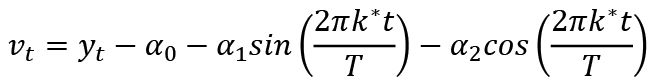(9)

The test statistics are calculated by estimating the following equation and using the error terms obtained in Eq. 9.

(10)

While the null hypothesis of this test denotes as H₀: α₁ = α₂ = 0, the alternative hypothesis denotes H₀: α₁ = α₂ ≠ 0. These hypotheses are examined by using the F test. After applying it, if the null hypothesis indicating the existence of a unit root is rejected, it can be said to be stationary around a deterministic function that breaks for the variables. The critical values calculated by Becker, Enders, and Lee are used for this test (Güriş, 2019: 3058). The other unit root test developed by Ranjbar et al. (2018) proposes a unit root test describing multiple smooth breaks against the symmetric or asymmetric (ESTAR) nonlinear alternative.

(11)

In Eq. 11, 𝛾 = [γ₁, γ₂] measures the width and displacement of the frequency component. If a structural break occurs, at least one of both frequency components must be present. In the optimal choice of k, the maximum k is only equal to 5. Based on the assumption and the deterministic components above, we test the following null hypothesis:

H₀: ε_t = υ_t, υ_t = υ_t–1 + u_t

Where assuming u_t is a zero-mean I(0) process. The null hypothesis is tested by Christopoulos and Leon-Ledesma’s (2010) critical values. In addition, Ranjbar et al. (2018) ascertained that their unit root testing approach is superior to Christopoulos and Leon-Ledesma’s (2010) test method. This ideal is based on both transition parameters, and the test power increases with frequency (Ranjbar et al., 2018).

3.2.2. Symmetric Causality Analysis

The causality aspect of the examined variables is crucial for almost all branches of science. In this respect, determining the direction of causality well is an eye-opener for the researchers. In the theory of econometrics, causality tests with various features have been developed. Symmetric causality analysis is also an improved form of the Toda-Yamamato (1995) causality test. Its distinctive aspect is the use of bootstrap simulation in the critical value generation process. The Modified Wald (MWALD) test was recommended by Toda and Yamamoto (1995) to test one of the variables over another variable in y_t where there is no Granger causality. The MWALD test statistic has an asymptotic χ²distribution with the number of degrees of freedom equal to the constraint number p. In addition, this test statistic is estimated to test the null hypothesis by generating a range of simulated observations. This hypothesis investigates whether y_2t is the Granger’s cause of y_1t or vice versa. If the hypothesis is rejected in terms of confidence intervals, it can be said that there is no relationship between the variables. In addition, it is suggested that this test is based on the asymptotic and bootstrap distribution. Asymptotic distribution may cause the test not to be the correct size for testing on finite samples. Herewith, the bootstrap distribution is seen as a suitable alternative instead of the asymptotic distribution against these said possible negativities (Hacker and Hatemi-J, 2006).

Efron (1979) is known to have explored the bootstrap method. The main idea of this method is based on resampling the data with the objective to estimate the statistical distribution. The decreasing skewness for more reliable critical values is a crucial rationale for using the bootstrap method. For Bootstrap simulations, initially, regression number 1 (y_t = v + A₁y_t–1 + ··· + A_py_t–p + ε_t) is estimated by the least squares method under the null hypothesis stating that there is no causal relationship. Accordingly, y^*_t, t = 1,… ,T; regression estimated coefficients ; The original data shows y_t–1,…, y_t–p and bootstrap residual. In Bootstrap simulation, the leverage vectors T×1 for y_1t and y_2t are written as t = 1,…,T, respectively, as follows (Hacker and Hatemi-J, 2006):

h₁ = diag(X₁ (X '₁ X₁)^–1X '₁) (12)

h₁ = diag(X(X 'X)^–1X ') (13)

Next, the modified residues for y_it are defined as:

After all, if the obtained MWALD test statistic value is greater than ‘bootstrap critical values’(c_α^*), it can be said that the null hypothesis based on the bootstrap is rejected, which indicates that there is a causality relationship between the variables (Hacker and Hatemi-J, 2006).

3.2.3. Hatemi-J (2012) Asymmetric Causality Analysis

Hatemi-J (2012) made a crucial contribution to the econometrics literature by revealing the causal link between negative and positive shocks to which the variables are exposed. This test uses the bootstrap simulation approach for the critical value generation process. The Hatemi-J (20212) information criterion is central in determining the optimal lag length (Hatemi-J, 2012: 450).

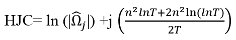(14)

In the equation 14, the symbol is the determinant of the predicted variance-covariance matrix of the error terms in the VAR model based on the j lag length; the notation n represents the number of equations in the VAR model, and T represents the number of observations. The test hypotheses are as follows: while the null hypothesis (H₀) states that there is no causality relationship between the variables, the alternative hypothesis (H₁) is vice versa.

The null hypothesis H₀: CB = 0 indicates that there is no Granger causality. This hypothesis is analyzed by the following test method (Hatemi-J, 2012: 451).

(15)

Where ⊕ represents the Kronecker product, symbol C represents the matrix p x n(1+np), and S_U denotes the variance-covariance matrix of the unrestricted VAR model.

4. Analysis Findings

In the symmetric causality test, the asymptotic distribution can produce erroneous results in finite samples, and the inferences made from this can be misleading. For this reason, it is considered appropriate to use the Bootstrap distribution, while considering that it can reduce the skewness in the results by providing more reliable critical values. The necessary value generation process was carried out in the asymmetric causality test with the Bootstrap simulation approach, similar to the symmetric causality analysis. The econometric model for research can be written as follows:

LNER_t = β₀ = β₁LNSTD_t + β₂LNUTD_t+ β₃NETRES_t + β₄NETCAP_t + β₅RIR_t + β₆LNCDS_t + β₇LNUNCt + ε_t (16)

Where β₀ and ε_tdenote the constant term and the error term, respectively. β₁, β₂, β₃, β₄, β₅, β₆ and β₇ illustrate slope coefficients. t indicates the time between 2008Q1 and 2020Q4. Table 2 presents the ADF Unit Root test results.

Table 2 indicates that NETRES, NETCAP, RIR, and LNUNC series are stationary at level values. The variables of LNER, LNSTD, LNLTD, and LNCDS are stationary when applying the first differences. Table 3 presents Phillips Perron (PP) unit root test results.

Table 2. Augmented Dickey-Fuller (ADF) Unit Root Test Results

Level	Variables	t-stat.	Prob.	Constant and Trend	Variables	t-stat.	Prob.
	LNER	1.025 (0)	0.996		LNER	-1.407 (0)	0.847
	LNSTD	-2.475 (0)	0.127		LNSTD	-1.342 (0)	0.865
	LNLTD	-0.765 (0)	0.820		LNLTD	-1.181 (0)	0.903
	NETRES	-4.748 (0)	0.003*		NETRES	-5.196 (0)	0.000*
	NETCAP	-7.733 (0)	0.000*		NETCAP	-7.732 (0)	0.000*
	RIR	-3.294 (1)	0.020*		RIR	-2.812 (1)	0.199
	LNCDS	-1.858 (0)	0.348		LNCDS	-2.907 (1)	0.170
	LNUNC	-4.980 (0)	0.001*		LNUNC	-5.107 (0)	0.000*
	∆LNER	-6.340 (0)	0.000*		∆LNER	-5.555 (4)	0.000*
	∆LNSTD	-5.838 (0)	0.000*		∆LNSTD	-6.041 (0)	0.000*
	∆LNLTD	-7.035 (0)	0.000*		∆LNLTD	-6.332 (0)	0.000*
	∆LNCDS	-5.926 (0)	0.000*		∆LNCDS	-5.37 (8)	0.000*

Note. The * symbol denotes statistically significant at 5% level. In addition, the values in parentheses ( ) state the lag length based on the Schwarz Info Criterion.

Table 3. Phillips Perron (PP) Unit Root Test Results

Level	Variables	Adj. t-stat	Prob.	Constant and Trend	Variables	Adj. t-stat	Prob.
	LNER	2.109 (8)	0.999		LNER	-1.049 (4)	0.927
	LNSTD	-1.906 (3)	0.326		LNSTD	-1.563 (3)	0.793
	LNLTD	-0.795 (0)	0.811		LNLTD	-1.368 (1)	0.858
	NETRES	-4.924 (0)	0.002*		NETRES	-5.300 (1)	0.000*
	NETCAP	-7.318 (5)	0.000*		NETCAP	-7.469 (7)	0.000*
	RIR	-3.002(5)	0.041*		RIR	-2.502 (6)	0.325
	LNCDS	-4.980 (1)	0.000		LNCDS	-5.121 (1)	0.000
	LNUNC	-4.980 (0)	0.001*		LNUNC	-5.107 (0)	0.000*
	∆LNER	-6.597 (5)	0.000*		∆LNER	-8.807 (11)	0.000*
	∆LNSTD	-5.058 (3)	0.000*		∆LNSTD	-5.016 (3)	0.000*
	∆LNLTD	-7.035 (0)	0.000*		∆LNLTD	-6.332 (0)	0.000*
	∆LNCDS	-5.831 (5)	0.000*		∆LNCDS	-6.187 (8)	0.000*

Note. The * symbol denotes statistically significant at 5% level. In addition, the values in parentheses ( ) state the Newey-West Bandwidth.

Table 3 indicates that the PP unit root test results are in line with ADF unit root test results. Accordingly, while the NETRES, NETCAP, RIR and LNUNC variables are stationary in their level values, other variables are stationary if the first difference is taken. Table 4 illustrates Kapetanios et al. (2003) nonlinear unit root test results.

Table 4. Kapetanios et al. (2003) Nonlinear Unit Root Test Results

Variables	Case 3	Case 2	Case 1
LNER	-1.87 (0)	1.05 (0)	2.97 (0)
LNSTD	-1.21 (1)	-1.73 (1)	1.46 (1)
LNLTD	-1.75 (0)	-1.42 (0)	1.75 (0)
NETRES	-0.03 (2)	0.05 (2)	0.26 (2)
NETCAP	-0.89 (2)	-0.89 (2)	-0.76 (2)
RIR	-2.25 (2)	-2.31 (2)	-2.06 (2)***
LNCDS	-3.24 (2)***	-3.38 (2)**	-0.69 (2)
LNUNC	-2.90 (2)	-2.90 (2)***	-2.96 (2)*
Critical Values
1%	-3.93	-3.48	-2.82
5%	-3.43	-2.93	-2.22
10%	-3.13	-2.66	-1.92

Note. Critical values were obtained from the article KSS (2003: 364). In addition, *, ** and *** symbols illustrate statistically significant at 1%, 5% and 10% levels, respectively. Raw data is represented by Case 1, while demeaned data is represented by Case 2. Finally, detrended data is represented by Case 3.

Table 4 indicates that the RIR variable is stationary at level values for Case 3 while LNCDS is stationary for Case 2, and Case 3. In addition, LNUNC is stationary for Case 1, and Case 2. Table 5 presents Sollis’s (2009) nonlinear unit root test results.

Table 5. Sollis (2009) Nonlinear Unit Root Results

Variables	FAE, t	FAEμ	FAE
LNER	1.84 (0)	4.30(0)***	6.75 (0)**
LNSTD	1.17 (1)	1.53 (1)	6.57 (0)**
LNLTD	1.55 (1)	1.31 (0)	2.02 (0)
NETRES	0.81 (2)	1.31 (2)	1.33 (2)
NETCAP	1.28 (2)	1.47 (2)	1.59 (2)
RIR	2.73 (2)	3.31 (2)	3.39 (2)
LNCDS	7.24 (2)**	6.02 (2)**	4.34 (2)***
LNUNC	13.34 (0)*	12.64 (0)*	4.57 (2)**
Critical Values
1%	8.79	6.89	6.78
5%	6.54	4.88	4.46
10%	5.41	4.00	3.57

Note. Critical values were obtained from Sollis (2009: 121) article. In addition, ** and *** symbols denote statistically significant at 5% and 10% levels, respectively. In these circumstances, it means that series are at stationarity. The zero mean is represented by FAE, while the non-zero mean is represented by FAE,μ,. Finally, the deterministic trend case is represented by FAE,t .

Table 5 indicates that the LNER, LNSTD, LNCDS, and LNUNC variables are stationary at level values. However, it was determined that other variables became stationary only after the first difference had been taken. Table 6 presents Kruse (2011) nonlinear unit root test results.

Table 6. Kruse (2011) Non-Linear Unit Root Test Results

Variables	Case 3	Case 2	Case 1
LNER	3.57 (0)	10.98 (0)**	15.17 (0)*
LNSTD	2.41 (1)	3.06 (1)	2.41 (1)
LNLTD	3.05 (0)	2.77 (0)	4.02 (0)
NETRES	1.29 (2)	1.85 (2)	1.45 (2)
NETCAP	2.12 (2)	2.15 (2)	1.69 (2)
RIR	5.46 (2)	6.08 (2)	5.31 (2)
LNCDS	11.46 (0)***	12.10 (2)**	8.77 (2)***
LNUNC	9.43 (2)***	8.24 (2)	8.99 (2)***
Critical Values
1%	13.15	13.75	13.15
5%	12.82	10.17	9.53
10%	7.85	8.60	7.85

Note. Critical values were obtained from the article Kruse (2011:6). In addition, * and ** symbols denote statistically significant at 1% and 5% levels, respectively. In these circumstances, it means that series are at stationarity. Raw data is represented by Case 1, while demeaned data is represented by Case 2. Finally, detrended data is represented by Case 3.

Table 6 indicates that the LNER, LNCDS and LNUNC variables are stationary at level values. However, the LNER variable is stationary for Case 1, and Case 2, while the LNUNC variable is stationary for Case 1 and Case 3. In addition, LNCDS is stationary for all cases. It was determined that other variables became stationary after taking the first difference. Table 7 presents Guris’s (2018) and Ranjbar’s (2018) Fourier Unit Root test results.

Table 7. Güriş (2019) ve Ranjbar (2018) Fourier Unit Root Test Results

	Variables	Level			Trend
		Test Sta.	k*	Lags	Test Sta.	k*	Lags
Güriş (2019)	LNER	32.64*	1	2	11.88	1	3
	LNSTD	11.30	1	4	32.15*	1	2
	LNLTD	16.08*	1	0	25.31***	1	1
	NETRES	2.76	2	4	1.45	1	4
	NETCAP	1.71	5	4	2.15	5	4
	RIR	6.17	1	4	3.77	1	4
	LNCDS	13.43***	1	2	11.51	1	2
	LNUNC	21.06*	1	0	20.48*	1	0
Ranjbar vd. (2018)	LNER	12.48*	1	2	6.25	1	3
	LNSTD	8.12**	1	4	15.59	1	1
	LNLTD	6.34***	1	0	11.90***	1	0
	NETRES	1.81	2	4	0.40	1	4
	NETCAP	5.80	1	4	2.88	1	4
	RIR	2.89	1	4	1.90	1	4
	LNCDS	7.69**	1	2	4.53	1	3
	LNUNC	14.23*	1	0	11.12**	1	2

Note: Guris (2019) and Ranjbar et al. (2018) articles were used for the critical values of the relevant tests. In addition, *, ** and *** symbols denote statistically significant at 1%, 5%, 10% levels, respectively. In these circumstances, it means that series are at stationarity.

Table 7 indicates that LNER, LNLTD, LNSTD, LNCDS and LNUNC variables are stationary at level values according to the critical values calculated by Guris (2019). Accordingly, it is proven that the null hypothesis has been rejected. Ranjbar et al.’s (2018) unit root test results show that LNER, LNSTD, LNLTD, LNCDS and LNUNC are stationary at level values according to the critical values calculated by Ranjbar et al. (2018). Therefore, it can be shown that Ranjbar et al. (2018) unit root test results are parallel to Güriş’s (2019) unit root test results. By examining other variables after the first difference was taken, it is proven that the other variables became stationary. It is revealed that linear and non-linear unit root tests give different results. Table 7 presents the symmetric causality analysis test results.

Table 8. Symmetrical Causality Test Results

Null Hypothesis (H0)	MWALD	Critical Values			Optimal Lags
		1%	5%	10%
LNER ≠> LNSTD	0.987	7.823	4.155	2.858	1
LNSTD ≠> LNER	2.886	7.398	4.133	2.888	1
LNER ≠> LNLTD	3.120***	7.897	4.421	3.109	1
LNLTD ≠> LNER	0.001	7.337	4.184	2.833	1
LNER ≠> RIR	0.527	7.220	4.033	2.806	1
RIR ≠> LNER	0.343	7.375	4.097	2.844	1
LNER ≠> NETRES	2.494	7.529	4.046	2.794	1
NETRES ≠> LNER	2.434	7.652	4.170	2.804	1
LNER ≠> NETCAP	2.745	7.381	4.090	2.854	1
NETCAP ≠> LNER	0.002	7.588	4.219	2.801	1
LNER ≠> LNCDS	0.107	7.122	4.039	2.812	1
LNCDS ≠> LNER	4.069***	7.328	4.189	2.912	1
LNER ≠> LNUNC	13.966*	8.431	4.229	2.800	1
LNUNC ≠> LNER	1.233	8.763	4.164	2.793	1

Note. The * and *** symbols indicate that the coefficients are statistically significant at 1%, and 10% levels, respectively. In these circumstances, it can be mentioned that there is a symmetric causality relationship between the variables. The bootstrap number is selected as 10,000. The Hatemi-J (2012) information criterion is used to determine the optimal lag length. ≠> displays no causality relationship.

Table 8 indicates a symmetric causality relationship between LNER to LNLTD, LNCDS to LNER, and LNER to LNUNC to reject the null hypothesis. It is known that if the calculated MWald test statistic is greater than the critical bootstrap values, the null hypothesis of non-Granger causality is rejected (Hacker and Hatemi, 2006). Accordingly, a unidirectional symmetrical causality relationship is determined from the exchange rate to the long-term debt stock, the credit default swap (CDS) to the exchange rate, and the exchange rate to the uncertainty index. Table 9 presents Hatemi-J (2012) Asymmetric Causality test results.

Table 9. Asymmetric Causality Test Results

Null Hypothesis (H0)	MWALD	Critical Values			Optimal Lags
		1%	5%	10%
LNSTD+≠>LNER+	0.058	8.286	4.582	3.188	1
LNSTD+≠>LNER–	14.494*	29.781	17.214	12.714	4
LNSTD–≠>LNER–	0.497	11.093	4.958	3.121	1
LNSTD–≠>LNER+	1.683*	22.385	12.848	9.620	4
LNLTD+≠>LNER+	0.662	7.974	4.388	2.996	1
LNLTD+≠>LNER–	0.121	13.247	5.492	3.352	1
LNER+≠>LNLTD–	4.457	8.909	4.550	3.093	1
LNLTD–≠>LNER–	0.090	11.161	4.930	3.074	1
LNLTD–≠>LNER+	1.903	12.301	5.289	3.273	1
RIR+≠>LNER+	0.209	11.509	4.675	2.942	2
RIR+≠>LNER–	3.010***	8.496	4.553	2.997	1
LNER+≠>RIR–	6.850**	11.332	5.107	3.097	1
RIR–≠>LNER–	0.000	9.450	4.480	2.979	1
RIR–≠>LNER+	2.248	9.023	4.418	3.023	1
NETCAP+≠>LNER+	0.000	10.781	4.998	3.285	4
NETCAP–≠>LNER+	0.170	11.890	5.032	3.229	4
LNER–≠>NETCAP+	5.403**	8.536	4.500	2.991	1
NETCAP–≠>LNER–	13.632*	11.632	5.191	3.264	1
NETCAP–≠>LNER+	1.683	11.600	4.798	2.975	1
NETRES+≠>LNER+	7.441**	10.408	4.879	3.176	1
NETRES+≠>LNER–	0.255	9.382	4.564	3.007	1
NETRES–≠>LNER–	0.561	9.249	4.630	3.106	1
NETRES–≠>LNER+	0.072	10.803	5.180	3.315	1
LNCDS+≠>LNER+	16.507*	12.300	5.417	3.387	1
LNCDS+≠>LNER–	0.201	9.957	5.141	3.320	1
LNCDS–≠>LNER–	0.420	10.063	5.041	3.411	1
LNCDS–≠>LNER+	0.617	8.522	4.638	3.124	1
LNUNC+≠>LNER+	9.463	42.956	20.761	14.927	1
LNUNC+≠>LNER–	7.779	44.068	22.908	16.474	1
LNUNC–≠>LNER–	2.880	45.511	22.586	15.752	1
LNUNC–≠>LNER+	4.726	42.731	22.164	15.728	1

Note. The *, ** and *** symbols indicate that the coefficients are statistically significant at 1%, 5% and 10% levels, respectively. The bootstrap number is selected as 10,000. The Hatemi-J (2012) information criterion is used to determine the optimal lag length. ≠> displays no causality relationship.

Table 9 indicates a causality relationship between positive shocks in the short-term debt stock to adverse shocks in the exchange rate. It is known that if the calculated Wald statistic is greater than the critical bootstrap values, the null hypothesis of non-Granger causality is rejected (Hatemi, 2012). Another result determines a causality relationship between positive shocks in the exchange rate to adverse shocks in the long-term debt stock. It proved bidirectional causality between positive shocks in the real interest rate to adverse shocks in the exchange rate and vice versa. In addition, another analysis results denote a causality relationship from adverse shocks in net capital investments to negative shocks in exchange rates. At the same time, there is a causality relationship between positive shocks in the net reserves to positive shocks in the exchange rate. In conclusion, the asymmetric causality relationship from positive shocks in CDS to positive shocks in the exchange rates is detected. This result reveals that the increase in the risk premium in the country raises the exchange rate.

5. Concluding Remark

This study investigates the causality relationship between the negative and positive shocks in the exchange rate and its factors after the 2008 global economic crisis. The maximum integration order has been determined based on the linear and nonlinear unit root test results. Next, symmetric causality analysis results indicate casualty relationship from the exchange rate to the long-term debt stock, from the credit default swap (CDS) to the exchange rate, and from the exchange rate to the uncertainty index. On the other hand, the asymmetric causality relationship provides information about the connection between the negative and positive shocks encountered by the variables. Accordingly, the first result shows a causality relationship between positive shocks in the short-term debt stock to negative shocks in the exchange rate. It has been revealed that short-term external debt stocks have a crucial impact on the exchange rate movements in Turkey which is among fragile countries. Another result is the causal relationship between positive shocks in the exchange rate and adverse shocks in the long-term debt stock. Despite employing different econometric methods, these results are in line with Akdoğan’s (2020) and Tatar and Erdogan’s (2020) analysis results. There is bidirectional causality from positive shocks in the real interest rate to adverse shocks in the exchange rate and vice versa. Similar results are determined in the following studies: Kayhan et al. (2013), Gök and Erkan (2021), and Karamelikli and Karimi (2022). In addition, results of other analyses indicate a causality relationship between negative shocks in the net capital investments to adverse shocks in the exchange rates. It is determined that negative shocks in the net capital investments, that is, capital outflows, may reduce the amount of the foreign exchange in the country, thereby leading to increases in the exchange rates. There is a causality relationship between positive shocks in the net reserves to positive shocks in the exchange rate. This result shows that an increase in the net foreign exchange reserves positively impacts national currencies. Bayat et al. (2014), Şit and Karadağ (2019), Çeştepe and Güdenoğlu (2020) studies detected a similar result to this finding. Finally, the asymmetric causality relationship from positive shocks in CDS to positive shocks in exchange rates is determined. In addition, Kar et al. (2016), Hassan et al. (2017), Münyas’s (2020) analysis results are in line with our findings despite employing different econometric methods.

6. Discussion

It is observed that the exchange rate fluctuations due to the abundance of global liquidity in the Turkish economy, like in other developing countries, were more stable between 2001–2013. Within this period, developed countries, especially the USA, implemented the expansionary monetary policy, and, with the contribution of financial asset purchases, international financial markets were significantly funded. However, this monetary abundance was reversed after 2013 with the high-interest policies of developed countries and the curbing of financial asset purchases. It could be said that this international conjuncture was one of the reasons for the rise in the exchange rates in Turkey. Other reasons have been related to Turkey’s economic and political structure. Here, in addition to the foreign trade deficit, the current account deficit, the debt stock, debt rollover rates, policy interest rates, inflation figures, and similar macroeconomic indicators, the independence of the Central Bank is questioned, policy decisions are unpredictable, risk and uncertainty are high, and the created political and legal instability were evaluated as other factors that increase the severity of fluctuations. If the Turkish economy fails to be one of the safe ports among the developing countries, the future of the exchange rate will continue to be affected by the aforementioned risks. This situation will bring along serious macroeconomic risks for a country that depends on imports for approximately 90% of its production.

References

Akduğan, U. (2020). Türkiye’de Döviz Kuru Hareketleri ve Kamu Borcu İlişkisi. Karadeniz Sosyal Bilimler Dergisi, 12(22), 75–97. https://doi.org/10.38155/ksbd.665188

Barbosa, L. O. S., Jayme Jr, F. G., & Missio, F. J. (2018). Determinants of the real exchange rate in the long run for developing and emerging countries: a theoretical and empirical approach. International Review of Applied Economics, 32(1), 62–83. https://doi.org/10.1080/02692171.2017.1332017

Bayat, T., Senturk, M., & Kayhan, S. (2014). Exchange rates and foreign exchange reserves in Turkey: nonlinear and frequency domain causality approach. Theoretical & Applied Economics, 21(11), 27–42.

Becker, R., Enders, W. and Lee, J. (2006). A Stationary Test in the Presence of an Unknown Number of Smooth Breaks. Journal of Time Series Analysis, 27(3), 381–409.

Benazic M. and Skabic K. I. (2016). The determinants of the exchange rate in Croatia, Eastern Journal of European Studies, 7(1), 125–150.

Çeştepe, H., & Güdenoğlu, E. (2020). Türkiye’de Döviz Rezervleri ve Döviz Kuru Arasındaki Asimetrik İlişkiİ: NARDL Yaklaşımı Bulguları. Mehmet Akif Ersoy Üniversitesi İktisadi ve İdari Bilimler Fakültesi Dergisi, 7(1), 231–251.

Chowdhury, M. and Hossain, Md. T. (2014). Determinants of Exchange Rate in Bangladesh: A Case Study. Journal of Economics and Sustainable Development, 5(1), 2014, Available at SSRN: https://ssrn.com/abstract=2668804.

Christopoulos, D.K. and León-Ledesma, M.A. (2010). Smooth Breaks and Non-linear Mean Reversion: Post-Bretton Woods Real Exchange Rates. Journal of International Money and Finance, 29(6), 1076–1093.

Dickey D. A., Fuller W. A. (1979). Distribution of the Estimators for Autoregressive Time 15 Series with a Unit Root. Journal of the American Statistical Association, 74(16), 427–431.

Dickey D. A., Fuller W. A. (1981). Likelihood Ratio Statistics for Autoregressive Time 13 Series with a Unit Root. Econometrica, 49(4), 1057–1072. https://doi.org/10.2307/1912517

Efron, B. (1979). Bootstrap methods: another look at the jackknife. Annals of Statistics, 7, 1–26.

Elfaki, K. E. (2018). Determinants of Exchange Rate Stability in Sudan (1991-2016). International Journal of Economics and Financial Issues, 8(2), 33.

Gök R. & Kara E. (2021). Testing for causality among cds, interest, and exchange rates: new evidence from the granger coherence analysis. Eskişehir Osmangazi Üniversitesi İktisadi ve İdari Bilimler Dergisi, 16(2), 427–445. https://doi.org/10.17153/oguiibf.854172

Granger, C. W. J. (1969). Investigating causal relations by econometric models and cross-spectral methods, Econometrica, 37, 424–38.

Granger, C. W. J. (1981). Some properties of time series data and their use in econometric model specification, Journal of Econometrics, 16, 121–30.

Granger, C. W. J. and Newbold, P. (1974) Spurious regression in econometrics, Journal of Econometrics, 2, 111–20.

Güriş B. (2019). A new nonlinear unit root test with Fourier function. Communications in Statistics - Simulation and Computation, 48(10), 3056–3062. https://doi.org/10.1080/03610918.2018.1473591

Hacker R. S. & Hatemi-J Abdulnasser (2006). Tests for causality between integrated variables using asymptotic and bootstrap distributions: theory and application. Applied Economics, 38(13), 1489–1500. https://doi.org/10.1080/00036840500405763.

Hassan, A., & Dantama, Y. U. (2017). Determinants of exchange rate volatility: new estimates from Nigeria. Eastern Journal of Economics and Finance, 3(1), 1–12.

Hassan, M. K., Kayhan, S., & Bayat, T. (2017). Does credit default swap spread affect the value of the Turkish LIRA against the US dollar? Borsa Istanbul Review, 17(1), 1–9. https://doi.org/10.1016/j.bir.2016.10.002

Hatemi-J. A. (2012). Asymmetric causality tests with application. Empir Econ, 43(1), 447–456, https://doi.org/10.1007/s00181-011-0484-x

He, Q., Liu, J., & Zhang, C. (2021). Exchange rate exposure and its determinants in China. China Economic Review, 65, 101579. https://doi.org/10.1016/j.chieco.2020.101579

Hepaktan E. (2009). Türkiye’nin Marshall-Lerner Koşuluna İlişkin Parçalı Eşbütünleşme Analizi, Yönetim ve Ekonomi Dergisi, 16(1), 39–55.

İlgün, M. F., Dumrul, C., & Ahmet, A. Y. S. U. (2014). Bütçe Açıklarının Reel Döviz Kuru Üzerindeki Etkileri: Türk Ekonomisi Üzerine Bir Uygulama. Uluslararası Yönetim İktisat ve İşletme Dergisi, 10(23), 13–30. https://doi.org/10.17130/ijmeb.2014.10.23.681

Kapetanios G., Shin Y. Snell A. (2003). Testing for a Unit Root in the Nonlinear STAR 28 Framework. Journal of Econometrics, 112(2), 359–379.

Kar, M., Bayat, T., & Kayhan, S. (2016). Impacts of credit default swaps on volatility of the exchange rate in Turkey: The case of Euro. International Journal of Financial Studies, 4(3), 14. https://doi.org/10.3390/ijfs4030014

Karamelikli, H., & Karimi, M. S. (2022). Asymmetric relationship between interest rates and exchange rates: Evidence from Turkey. International Journal of Finance & Economics, 27(1), 1269–1279.

Kayhan, S., Bayat, T., & Ahmet, U. (2013). Interest rates and exchange rate relationship in BRIC-T countries. Ege Academic Review, 13(2), 227–236.

Kruse, R. (2011). A New Unit Root Test against ESTAR based on a Class of Modified 30 Statistics. Statistical Papers, 52, 71–85.

Makhdom, M. A. (2021). Makroekonomik Göstergeler İle Döviz Kuru Arasındaki İlişkinin Analizi: (2005:01-2019:10) Türkiye Uygulaması. İşletme Araştırmaları Dergisi, 13(1), 772–789.

Mungule, K. O. (2020). The determinants of the real exchange rate in Zambia (Doctoral dissertation, AERC).

Münyas, T. (2020). Evaluation of the Relationship between Credit Default Swaps and EURO and USD Exchange Rates: The Case of Turkey. Business & Management Studies: An International Journal, 8(2), 1113–1130.

Oriavwote E. V. ve Oyovwi O. D. (2012). The Determinants of Real Exchange Rate in Nigeria, International Journal of Economics and Finance, 4(8).

Perron, P. (1989). The Great Crash, The Oil Price Shock, and The Unit Root Hypothesis. Econometrica, 57, 1361–1401.

Phuc, N. V., & Duc, V. H. (2021). Macroeconomics determinants of exchange rate pass-through: new evidence from the Asia-Pacific region. Emerging Markets Finance and Trade, 57(1), 5–20. https://doi.org/10.1080/1540496X.2018.1534682

Raksong, S., & Sombatthira, B. (2021). Econometric Analysis of the Determinants of Real Effective Exchange Rate in the Emerging ASEAN Countries. The Journal of Asian Finance, Economics and Business, 8(3), 731–740. https://doi.org/10.13106/jafeb.2021.vol8.no3.0731

Ranjbar, O., Chang, T., Elmi, Z., Lee, C. (2018). A New Unit Root Test against Asymmetric ESTAR Nonlinearity with Smooth Breaks. Iranian Economic Review, 22(1), 51–62. https://dx.doi.org/10.22059/ier.2018.65349

Raza, S. A., & Afshan, S. (2017). Determinants of exchange rate in Pakistan: Revisited with structural break testing. Global Business Review, 18(4), 825–848. https://doi.org/10.1177%2F0972150917692210

Saeed, A., Awan, R.U., Sial, M.H., & Sher, F. (2012). An Econometric Analysis of Determinants of Exchange Rate in Pakistan. International Journal of Business and Social Science, 3(6) [Special Issue -March 2012].

Şarkaya I., C. (2019). Reel Efektif Döviz Kurunu Belirleyen Ekonomik Faktörlerin Araştırılması: Heterojen Panel Veri Analizi. Mehmet Akif Ersoy Üniversitesi İktisadi ve İdari Bilimler Fakültesi Dergisi, 6 (3), 736–749. https://doi.org/10.30798/makuiibf.570833

Şimşek M. (2004). Türkiye’de Reel Döviz Kurunu Belirleyen Uzun Dönemli Etkenler. İktisadi ve İdari Bilimler Fakültesi Dergisi, 1–24.

Şit, M. ve Karadağ H. (2019). Döviz Kurunu Belirleyen Ekonomik Faktörler: Türkiye Ekonomisi için ARDL Sınır Testi. International Journal of Economic & Administrative Studies, 23, 151-167. https://doi.org/10.18092/ulikidince.476930

Sollis R. (2009). A Simple Unit Root Test against Asymmetric STAR Nonlinearity with an 8 Application to Real Exchange Rates in Nordic Countries. Economic Modelling, 26(9), 118–125.

Suthar, Mita H. (2008) Determinants of Exchange Rate in India (April 21, 2008). Available at SSRN: https://ssrn.com/abstract=1165602 or http://dx.doi.org/10.2139/ssrn.1165602

Tatar E., H. ve Erdoğan, S. (2020). Türkiye’de Döviz Kuru ve Dış Borç İlişkisi. Uluslararası Yönetim İktisat ve İşletme Dergisi, 16(1), 47–61. https://doi.org/10.17130/ijmeb.700844

Toda, H. Y., and Yamamoto, T. (1995). Statistical inference in vector autoregressions with possibly integrated processes. Journal of Econometrics, 66, 225–50. https://doi.org/10.1016/0304-4076(94)01616-8