Ekonomika ISSN 1392-1258 eISSN 2424-6166
2023, vol. 102(1), pp. 60–80 DOI: https://doi.org/10.15388/Ekon.2023.102.1.4
Gamze Kılınç
Suleyman Demirel University, Social Sciences Institute, Department of Business
In the Logistics Subfield YÖK 100/2000 and TÜBİTAK PhD Scholar, Isparta, Turkey
Email: gamzeeklncc@gmail.com
ORCID: https://orcid.org/0000-0001-7746-3634
Turan Kocabıyık
Suleyman Demirel University, Faculty of Economics and Administrative Sciences
Finance and Banking Department, Isparta, Turkey
Email: turankocabiyik@sdu.edu.tr
ORCID: https://orcid.org/0000-0003-3651-206X
Meltem Karaatlı
Suleyman Demirel University, Faculty of Economics and Administrative Sciences
Department of Business, Isparta, Turkey
Email: meltemkaraatli@sdu.edu.tr
ORCID: https://orcid.org/0000-0002-7403-9587
Abstract. BDI is a global trade indicator followed by those interested in maritime trade. But it has volatility, seasonality, and uncertain cyclicality. For this reason, in this study, the BDI has been estimated to provide preliminary information to those interested in maritime trade. NARX Neural Network which performs successfully in complex and nonlinear real-life problems is used. In addition, the NARX neural network model has not been found in a previous study used for BDI estimation. Eleven independent variables are used in this study, what increases the predictive power. Independent variables are Bloomberg Commodities Index (BCOM), Twitter-Based Economic Uncertainty Index (TEU), Twitter-Based Market Uncertainty Index (TMU), S&P 500 Index, MSCI World Index, €/$ Parity, VIX (CBOE), US 10-Year Bond Yield (%), Brent Oil (USD/Barrel), Economic Uncertainty Index and World Trade Volume (USD Billion). The Twitter-Based Economic Uncertainty Index (TEU) and Twitter-Based Market Uncertainty Index (TMU), which were not used before in BDI estimation studies, were included in the analysis and contributed to the literature. The data set contains daily data for the period 9.07.2012–31.08.2020. 11-day estimate values covering 1.09.2020–15.09.2020 are calculated. MAPE, MAE and RMSE performance criteria were calculated for the estimation values. Value of MAPE (2.96%), value of MAE (36.6%) and value of RMSE (46.68) were obtained. As a result, the estimate values were compared with the actual values.
Keywords: NARX Neural Networks, Baltic Dry Index, Estimate
_____________
Received: 18/07/2022. Revised: 17/10/2023. Accepted: 13/01/2023
Copyright © 2023 Gamze Kılınç, Turan Kocabıyık, Meltem Karaatlı. Published by Vilnius University Press
This is an Open Access article distributed under the terms of the Creative Commons Attribution License, which permits unrestricted use, distribution, and reproduction in any medium, provided the original author and source are credited.
Today, with the rapid development of technology, global trade has gained momentum. It has brought elements such as strict price policies, flexible response ability, and quality competition. The importance of global trade and trade competition elements is gradually increasing in order to respond accurately and timely to the needs arising from rapidly advancing technological developments and increasing living standards. In this direction, maritime transportation is the most used transportation type among the global trade transportation types with a rate of 90 percent. However, the growth in international maritime trade has come to a standstill as of 2019, showing the lowest values since the global financial crisis of 2008–2009. At the same time, global trade in goods contracted by 0.5 percent due to high policy uncertainty, supply chain disruptions, and demand contractions caused as a result of trade tensions. The global health threat and economic crisis posed by the COVID-19 epidemic, which emerged at the end of 2019, adversely affected maritime trade. Therefore, the global trade sector has been faced with the negative effects of both the changing demands of the globalizing world and the uncertain supply-demand balances in the pandemic environment (Trujillo and Tovar, 2007; UNCTAD, 2020). In this regard, it is extremely important to predetermine the situations affecting the trade activities in the global market and to create a business plan.
The Baltic Exchange, located in London, aims to standardize the freight prices given to shipping companies in maritime transport. For this reason, daily data on dry cargo types are published under the name of Baltic Dry Index. The Baltic expression in the name of the index indicates that it is calculated by the Baltic Stock Exchange. However, it should not be ignored that BDI values are not limited to only Baltic Sea countries or a few commodities. Baltic Dry Index is a freight price index calculated according to the values of many commodities such as coal, iron ore, grains, etc. on 23 different routes. BDI concerns not only ship owners and charterers, but also companies operating in the logistics and financial fields through maritime transport around the world. For this reason, it is an index accepted as an indicator of global trade. Due to the fact that it is an indicator that is followed on a global scale, it is affected by many different factors such as supply, demand, political and economic factors in worldwide. Therefore, it is a time series with high volatility and uncertainty. Determining the dynamics and trends of this index is very important for companies in risk control and planning (Barut et al., 2020; Zeng and Qu, 2014).
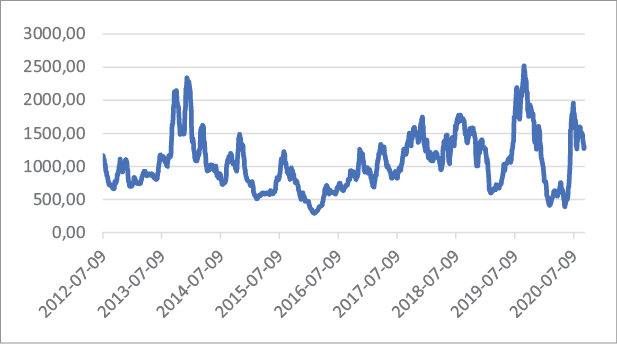
The Baltic Dry Index is an econometric indicator that is closely influenced by the internal dynamics of maritime transport. Therefore, all companies, businesses, shipowners, investors, etc. operating in maritime transport, professional groups follow it closely. However, the seasonality, nonstationary nature and uncertain cyclicality of the Baltic Dry Index given in Figure 1 make it difficult to predict. For this reason, there are various studies on the BDI index and its estimation in the academic world (Lin and Wang, 2014; Papailias et al., 2017).
Traditional econometric methods have poor performance in estimating high volatility time series. In the comparative analysis studies of Artificial Neural Networks (ANN) method and traditional estimation methods in the literature (Alon et al., 2001; Sahin, 2018), it is seen that ANN performs better in nonlinear time series with variable structure. Because the ANN method is very successful in solving complex situations in real life, due to its nonlinear structure, tolerance of error and noise, processing fuzzy and probabilistic information, and learning and generalization abilities. With network training, it makes estimations by acting like biological neurons in the human body, generalizing from experiences (dependent variables) to unknown (independent) variables (Basheer and Hajmeer, 2000). However, it has some disadvantages. ANNs are hardware-dependent and network training takes time. The creation of the appropriate network structure and the determination of the parameters is carried out by the trial and error method (Sert, 2014). However, it has been determined that NARX networks, one of the artificial neural networks, outperform NAR neural networks (Yang and Mehmed, 2019). For this reason, in this study, the estimation of the Baltic Dry Index was carried out with the NARX Neural Network. This study has two important differences from other studies. The first is rich variable coverage, which increases predictive power. Secondly, no study was found that included the analysis of BDI with the NARX neural network model. The 11 explanatory variables used in the analysis cover many of the various variables that have been identified in both econometric models and estimating models in the literature. At the same time, it prepares the infrastructure for a detailed and realistic analysis by including the variables newly added to the literature for a more accurate estimation of the BDI. The study has been enriched by including the Twitter-Based Economic Uncertainty Index (TEU) and Twitter-Based Market Uncertainty Index (TMU), which have not been used before in BDI estimation studies. Although there are studies that analyze BDI with ANN, a study that makes estimations using the Nonlinear External Input Autoregressive NARX neural network model of the ANN method has not been found in the literature. Jeong and Park (2017) showed that the potential of NARX neural networks for short-term electric charge estimation is higher than that of NAR and statistical estimation methods. As a result, he found NARX more suitable for the prediction of dynamic structures. For this reason, NARX neural networks have been found suitable for the prediction of the dynamic structure of BDI. In these aspects, the study differs from other studies.
The remainder of this paper is organized as follows. Section 2 includes information about the Baltic Dry Index. Section 3 presents literature reviews. In Section 4, purpose, data set, methodology, empirical results, and discussion are given under the title of the application, respectively. Finally, in Section 5 the results, evaluations, and suggestions are given.
Businesses and investors interested in maritime transport consider the balance of supply, demand, and cost in the trade of goods to be transported for a healthy logistics activity. For this reason, it has been observed that there is a directly proportional relationship between the number of goods whose logistics are carried out and the development of global and regional trade activities (Kiraci and Akan, 2020). However, to demonstrate this relationship more clearly, the Baltic Freight Index (BFI) was created by the London Baltic Exchange in 1985. The BFI was initially evaluated with an index base score of 1000. It continued to be published as the Baltic Dry Index (BDI) in 1999. The London Baltic Exchange provides an independent maritime trade database. It provides an independent database of maritime trade by hosting more than 3000 international communities. Members of the Baltic Exchange consist of shipowners, shipbrokers, ship charterers, maritime lawyers, arbitrators, P&I (Protection and Indemnity) Insurance Clubs, and other maritime associations. BDI is a composite index calculated based on the tonnage, numbers, routes, Cargo, and price of the Handysize, Supramax, Panamax, and Capesize bulk carriers. The index value is intended to be a representation of freight prices for reconciliation in freight derivative transactions. Because the freight rates requested by the shipowners for the charter of ships are also an indicator of the financial fluctuations in maritime transport, BDI is an index that quickly reflects the dynamics of global commercial activities, as it is published daily. Thus, it is a leading indicator as it offers a more agile forecasting opportunity compared to growth-oriented macroeconomic data. The increase or decrease of the index is directly proportional to the increasing or decreasing demand in global commercial activities. For this reason, the course of the index guides investors in terms of global supply-demand, economic growth, and contractions. Investors get preliminary information by researching long-term trends and unusual changes along with their reasons on the index. In the light of the information they interpret, they have the opportunity to take a more secure position for the future. Ship brokers, ship owners, operators, traders, financiers and charterers benefit from BDI values (Baltic Exchange, 2021; Culline et al., 1999; Ruan, et al., 2016). BDI is a value that includes shipping costs incurred in trading various raw materials such as metals, grains, and fossil fuels transported by sea. This global trade index is calculated by considering the freight rates applied on important trade routes. It is calculated with a certain weighting after the average of the freight values sent by the panel members of the Baltic Exchange in London. However, the lowest and highest freight values from each trade route are excluded from the calculation so that the index value is not subject to any speculation. For this reason, BDI is a leading indicator for global trade, with both extensive coverage and a reliable and independent database (Baltic Exchange, 2021; Culline et al., 1999).
The Studies on BDI where ANN is not used. Yılmazkuday (2020) examined the effects of deaths from COVID-19 disease on BDI and crude oil prices. While a decrease was observed in BDI values, there was no significant effect on crude oil prices. Bakshi et al. (2010) determined that global stock market returns, commodity index returns, and the growth rate in global real economic activity are related to the BDI growth rate. Lin and Wang (2014) propose a model that best predicts a dynamic structure of BDI with fuzzy set theory, gray system theory, and traditional time series models. Papailias et al. (2017) concluded that the trigonometric regression model performs best in predicting the cyclical change of BDI. Cihangir (2018) found that the effects of the VIX volatility index on BDI are positive and statistically significant in the short and long terms. Zeren and Kahramaner (2019) concluded that BDI and ISTFIX (Istanbul Freight Index) are acting together and that BDI is directing ISTFIX in the long term. Kiraci and Akan (2020) examined the symmetric and asymmetric causality between BDI, oil prices, and the dollar index.
The Studies on ANN and Comparative studies of ANN with other estimation methods. Lin et al. (1996) concluded that the NARX neural network structure can store 2 to 3 times more information than traditional neural networks. Siegelmann et al. (1997) concluded that the NARX neural network model, which has a gradient descent learning structure, is more effective than the artificial neural network model in long-term problems. Mitrea et al. (2009) found that the artificial neural network model performance is better than Moving Average (MA) and Autoregressive Integrated Moving Average (ARIMA). Zeng et al. (2014) compared EMD-ANN (Empirical Mode Decomposition-Artificial Neural Networks), EEMD-ANN (EMD-Artificial Neural Networks with compositional process), ANN (Artificial Neural Networks) and VAR (Vector Automatic Regression) models. They concluded that the best performing model was the EMD-ANN model developed in this study.
The Studies in which ANN and BDI are used together. By Sahin et al. (2018), as a result of three different ANN models, it was concluded that COP (Crude Oil Prices) did not affect BDI, but ANN model was effective in BDI estimation performance. Chou and Lin (2019) examined BDI with a fuzzy neural network model combined with technical indicators to determine the freight rate trend.
The Studies involving the variables used in this study. In the literature, econometric models have been established to increase the predictability of the dynamic structures of BDI and their relations with various variables have been tried to determine. Han et al. (2020) found that the long-term predictability of BDI using exchange rates with panel regression analysis gave meaningful results. Ruan et al. (2016) found that the relationship between BDI and crude oil prices was statistically significant with the cross-correlation statistical test and multi-fractal cross-correlation analysis (MF-DCCA). Bildirici et al. (2015) found a positive relationship between BDI and economic growth through the VAR model on the USA sample. Other types of studies in the literature are BDI estimation studies. Sahan et al. (2018) proposed a BDI estimation model with Integrated Autoregressive Moving Average (ARIMAX). They used commodity price index for metals, price index for food, crude oil prices, 10-year US bond yield, world industrial production S&P 500 index, world consumer price index, gold spot prices, silver spot prices, and US dollar exchange rate as independent variables.
In this study, the Baltic Dry Index, which is of great importance in maritime transport activities and has high volatility, was estimated by NARX neural network model in order to determine the dynamics and trends. The estimation of the Baltic Dry Index will help people and businesses dealing with maritime transport to realize their business plans in a more controlled manner.
BDI is affected by many factors as it is a global indicator of maritime trade. In this study, the selection of variables was carried out by taking into account the studies that were found to be related in the literature. However, two independent variables that were not found to be used in BDI estimation studies before were included in the analysis. These are the Twitter-Based Economic Uncertainty Index (TEU) and the Twitter-Based Market Uncertainty Index (TMU) to represent uncertainty.
Twitter is a social platform where people can share their feelings, situations, and thoughts instantly. The widely used social platform Twitter is a database containing not only the opinions of experts but also the society. Baker et al. (2021) observed the economic uncertainty in real-time, created the Twitter-Based Economic Uncertainty Index (TEU) and the Twitter-Based Market Uncertainty Index (TMU) over tweets containing keywords such as “uncertainty in the economy”, “uncertainty”, “economy”. While creating the index, to understand the effect of any tweet, the number of retweets is used. Weight coefficients are created with this number and index values are determined. Wu et al. (2021) in their studies, using the Twitter-Based Economic Uncertainty Index (TEU) and the Twitter-based Market Uncertainty Index (TMU), examined the effects of economic policy uncertainty on the cryptocurrency markets. Aharon et al. (2021) in their studies, using TEU and TMU variables, examined the relationship between uncertainties and cryptocurrencies. In this study, the Twitter-Based Economic Uncertainty Index (TEU) and Twitter-Based Market Uncertainty Index (TMU) were included in the analysis in order to represent uncertainty among the explanatory variables of BDI and to improve estimate performance.
In this study, eleven independent variables, which were directly or indirectly related in BDI, were determined as a result of the literature review. Bloomberg Commodities Index (BCOM), Twitter-Based Economic Uncertainty Index (TEU), Twitter-Based Market Uncertainty Index (TMU), S&P 500 Index, MSCI World Index, €/$ Parity, VIX (CBOE), US 10-Year Bond Yield (%), Brent Oil (USD/Barrel), Economic Uncertainty Index and World Trade Volume (USD Billion) were used as input variables, Baltic Dry Index was used as output variable. The data set consists of daily data for the period 9.07.2012–31.08.2020. Since the BDI values only include weekdays, the data set was arranged as five days a week. Databases from which variables are obtained, links, access dates, and sources are given in Table 1.
|
Data |
Link |
Access Date |
Source |
|
Baltic Dry Index (BDI) |
18.03.2021 |
||
|
Bloomberg Commodity Index (BCOM) |
https://tr.investing.com/indices/bloomberg-commodity-historical-data |
18.03.2021 |
|
|
Twitter-Based Economic Uncertainty Index (TEU) |
18.03.2021 |
Economic Policy Uncertainty Web Page |
|
|
Twitter Based Market Uncertainty Index (TMU) |
18.03.2021 |
Economic Policy Uncertainty Web Page |
|
|
S&P 500 Index |
19.03.2021 |
||
|
MSCI World Index |
18.03.2021 |
||
|
€/$ Parity |
18.03.2021 |
TCMB |
|
|
VIX (CBOE) |
https://tr.investing.com/indices/volatility-s-p-500-historical-data?cid=1096487 |
19.03.2021 |
|
|
US 10-Year Bond Yield (%) |
https://tr.investing.com/rates-bonds/u.s.-10-year-bond-yield-historical-data |
18.03.2021 |
|
|
Brent Oil (USD/Barrel) |
https://www.matriksdata.com/website/-kurumsal-urunler/matriks-prime |
18.03.2021 |
Matrix Prime Program |
|
Economic Uncertainty Index |
23.03.2021 |
Economic Policy Uncertainty Web Page |
|
|
World Trade Volume (USD Billion) |
02.04.2021 |
The Netherlands - Centraal Planbureau (CPB) - Bureau for Economic Policy Analysis (Web Page) |
Descriptive statistics of dependent and independent variables are given in Table 2.
|
N |
Maximum |
Minimum |
Mean |
Std. Deviation |
Variance |
|
|
Baltic Dry Index (BDI) |
2135 |
2518.00 |
290 |
1054.34 |
422.76 |
178729.22 |
|
Bloomberg Commodity Index (BCOM) |
2135 |
152.01 |
59.48 |
98.14 |
23.88 |
570.30 |
|
Twitter-Based Economic Uncertainty Index (TEU) |
2135 |
2265.01 |
17.13 |
148.67 |
140.12 |
19634.17 |
|
Twitter Based Market Uncertainty Index (TMU) |
2135 |
1958.64 |
14.46 |
152.00 |
128.32 |
16466.21 |
|
S&P 500 Index |
2135 |
3580.84 |
1334.76 |
2283.18 |
520.74 |
271165.26 |
|
MSCI World Index |
2135 |
2494.10 |
1201.74 |
1823.73 |
284.83 |
81128.78 |
|
€/$ Parity |
2135 |
1.40 |
1.04 |
1.19 |
0.10 |
0.01 |
|
VIX (CBOE) |
2135 |
82.69 |
9.14 |
16.29 |
6.96 |
48.41 |
|
US 10-Year Bond Yield (%) |
2135 |
3.24 |
0.52 |
2.16 |
0.58 |
0.33 |
|
Brent Oil (USD/Barrel) |
2135 |
118.87 |
19.03 |
70.90 |
25.53 |
651.87 |
|
Economic Uncertainty Index |
2135 |
298.00 |
140 |
174.37 |
23.46 |
550.60 |
|
World Trade Volume (USD Billion) |
2135 |
126.97 |
104.1987 |
116.33 |
6.46 |
41.72 |
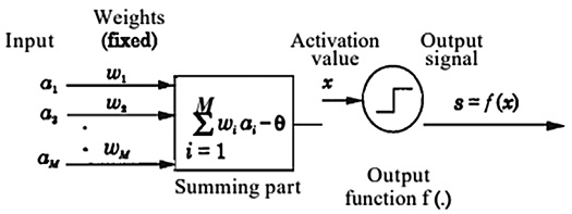
Artificial neural networks (ANN) are mathematical modeling of the learning process inspired by the human brain. The general architecture of artificial neural networks is given in Figure 2. ANN are weighted directed structures between inputs and outputs with artificial neurons. ANNs are generally divided into two groups as feedforward networks and feedback networks. Feedforward networks have a static structure. Networks of this nature calculate the output response to the input independently of the previous inputs. It does not have a loop structure that can give feedback between units. Information in this network structure moves forward through the input layer, hidden layer, and output layers, respectively. For this reason, it has a memoryless network structure. Feedback networks, on the other hand, have a dynamic structure. In networks with this structure, an output is obtained depending on both the current and previous inputs. This shows that the network has a memory with a circular structure (Jain et al., 1996).
ANN has several advantages compared to other estimation methods in terms of successful fault tolerance, flexibility in network structure, and working with different structures (fuzzy, probabilistic, noisy data structures) (Yegnanarayana, 2009).
Each piece of information coming to artificial neurons is weighted according to its importance. It is aimed to minimize the error. For this reason, the learning cycle continues until the best weighting coefficients are obtained. The activation function has an important place in the realization of learning, because an artificial neural network built without using the activation function will exhibit a structure similar to the linear regression model.
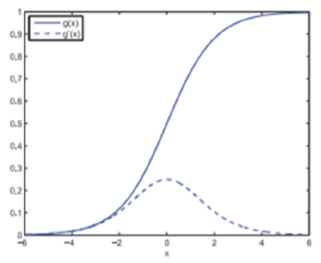
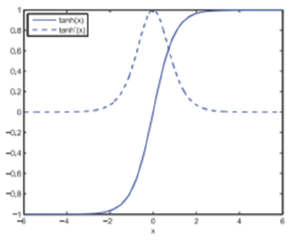
There are various activation functions with different properties. In order to minimize the error, nonlinear and differentiable activation functions are preferred. These are the sigmoid and tangent hyperbolic functions. Its mathematical equations are given by Equation (1) and (2), respectively. The sigmoid graph and its derivative and the tangent hyperbolic graph and its derivative are given in Figure 3 and Figure 4, respectively. The fact that these functions are nonlinear and continuous, that is, differentiable, play an important role in learning and estimating complex data. As seen in Figure 3, the sigmoid function takes probabilistic values in the range of [0,1]. The disadvantage of this function is the “disappearing gradient” problem. This problem occurs when the sigmoid derivative function converges to 0 at extreme values. In this case, learning takes place at a minimum level. As seen in Figure 4, the tangent hyperbolic function takes values in the range of [-1,1]. Since its derivative is steeper than the sigmoid function, the range of values is wider. This allows for faster learning. However, similar to the sigmoid function, gradient dying is encountered at the endpoints (Ding et al., 2018).
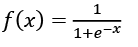 (1)
(1)
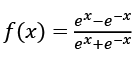 (2)
(2)
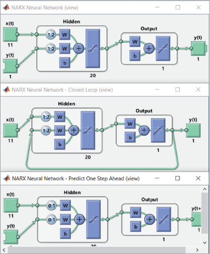
The Nonlinear External Input Autoregressive Network (NARX) model used in this study has a recurrent neural network structure (Siegelmann et al., 1997). The general architecture of the NARX Neural Network is given in Figure 5. The network structure gains degrees of freedom and decreases the number of parameters within the information coming from exogenous inputs. Thus, different models can be realized with the same information. NARX structure is mathematically given by Equation (3) below
y(t) = f(y(t – 1), y(t – 2),…,y(t – ny), u(t – 1), u(t – 2),…, u(t – nu)) (3)
where y(t) is dependent variable, y(t – ny) ∈ R represents the network output, u(t – nu) is the network input, ny and nu represent the number of past outputs and past inputs to be applied for feedback, respectively (Chaudhuri and Ghosh, 2016; Guzman et al., 2017).

For learning to occur, each neuron in the NARX neural network produces an output that is fed back from the output layer to the input layer by the sigmoid activation function. The nonlinear sigmoid activation function can backpropagate with its differentiability feature. The error values calculated as a result of the neural networks feedforward are the estimation values and are reused for the next prediction in parallel structure. Thus, the error values reach the smallest possible value with the backpropagation algorithm. At the same time, this serial-parallel network structure reduces recurrent time. As a result, NARX neural network starts with random weighting and reaches the optimum result with a serial-parallel network structure (Guzman et al., 2017).
The Levenberg–Marquardt (LM) algorithm, developed by Levenberg (1944) and Marquardt (1963), provides a numerical solution for the minimization of nonlinear functions. This algorithm gives more stable and faster results with the combination of the gradient descent method and Gauss–Newton method for training neural networks (Yu and Wilamowski, 2018). For this reason, the Levenberg–Marquardt (LM) algorithm was used in this study.
There are various model selection criteria in the literature. The Schwarz Information Criterion (SIC) has a more flexible and successful structure for adding new variables to the model compared to the Akaike Information Criterion (AIC). For this reason, SIC was used in this study (Ucal, 2006).
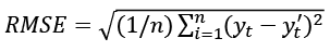
Various performance measures are used to measure the predictive accuracy (prediction performance) of the models. The main performance measures commonly used in the literature are Mean Absolute Percentage Error (MAPE), Mean Square Error (MSE), Mean Absolute Error (MAE), and Root Mean Square Error (RMSE). These criteria are given by Equations 4, 5, 6, and 7 (Bolzan et al., 2008):
 (4)
(4)
 (5)
(5)
 (6)
(6)
 (7)
(7)
where yt represents the actual value, yt' is the estimate value and n is the number of samples. According to Lewis (1982), models with a MAPE value below 10% are “very good”, models between 10% and 20% are “good”, models between 20% and 50% are “acceptable”, models belove 50% are “wrong and faulty” classified. The mean size of the errors in the estimation is calculated with the MAE and the standard deviation with the RMSE. These criteria can take values in the range (0, ∞).
In the NARX neural network model, the nonlinear relationship between the input and output variables and the number of neurons is directly proportional. If the number of hidden layers used is low, the network cannot fully learn. On the contrary, if more hidden layers are used than necessary, the network performs overfitting. Thus, the generalization ability of the network is negatively affected. In the NARX neural network model, the data coming from the input layer is processed in the hidden layers and sent to the next layer. All hidden layers have more than one processor element in the model. In the literature, the number of hidden layers and the number of processor elements are determined by the users by the trial and error method. For this, the user tries the number of neurons in an increasing order starting from a small value and accepts the number of neurons as the optimum value when the network achieves the best performance (Bayir, 2006).
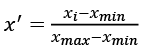
In order to prepare artificial neural networks for training and to determine their architecture, the data must first be normalized (Guzman et al., 2017). In this study, the data set was normalized by taking values in the range of (0,1) with the min-max normalization method. Min-max normalization is given by Equation (8) (Larose, 2005).
 (8)
(8)
In Equation 8, x' represents the normalized data, xi represents the input value, xmin represents the smallest number among the input values, xmax is the largest number among the input values.
In this study, experiments were carried out to find the best performance of the NARX neural network model for the Baltic Dry Index with different training, validation, test percentages, and different neuron numbers. The experiments were carried out with MATLAB program. The results of experiments are given in Table 3. The training dataset is the set created to determine the data and make predictions on this data in order to train the algorithm. The validation dataset is a subset of data used to evaluate the performance of the model obtained during the training phase. The test dataset is a dataset used to evaluate the model developed in the training set. With the MAPE performance value, which is one of the performance criteria, it was decided that the network showed the best performance when 60% training, 20% validation, 20% testing, and 20 neurons were used. The lag coefficient was accepted as 2 according to the Schwarz information criterion (SIC). Lags refer to the association of values within a time series with previous copies of itself. The lag coefficient is the lag time constant.
|
Data Set (Divided into 3 Groups in Percentages) |
60% education |
70% education |
80% education |
|||||||||
|
Number of Neurons |
15 neurons |
20 neurons |
25 neurons |
30 neurons |
15 neurons |
20 neurons |
25 neurons |
30 neurons |
15 neurons |
20 neurons |
25 neurons |
30 neurons |
|
MAPE |
5.09 |
2.98 |
5.55 |
4.79 |
4.64 |
3.64 |
4.07 |
5.87 |
3.03 |
7.30 |
4.91 |
4.56 |
Parallel and serial architectures of the NARX neural network are given in Figure 6. Here, x(t) refers to eleven independent variables and y(t) refers to one dependent variable. In the NARX neural network model, the input layer, the hidden layer, and the output layer are seen respectively. There are twenty neurons in the hidden layer and one neuron in the output layer. At the same time, activation functions contribute to the emergence of more successful results by learning the complex structures of the datasets in a better way.
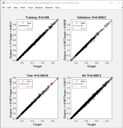
Training, validation, and test success in the created NARX neural network model are given in Figure 7 with the regression graph. Values of the correlation coefficient (R) measure the correlation between output and goals. R value of 1 means a close relationship, and 0 means a random relationship. Values between outputs and targets are very close to “1”. The general correlation coefficient of the dataset was obtained as 0.99872.
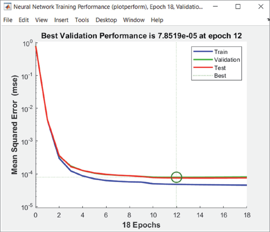
The performance of the NARX neural network is measured by MSE (Mean Square Error). MSE refers to the mean square difference between outputs and targets. As the MSE value approaches zero, the success rate increases. A value of zero means that there is no error. The MSE values and performance graph at each step of the model created are given in Figure 8. As can be seen, the lowest MSE value was obtained in the 12th iteration of the training, which was completed in 18 iterations. Also, the NARX neural network performed the best validation and performance at this stage.
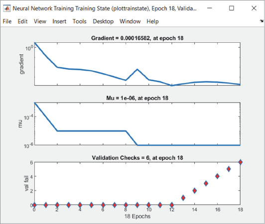
The output graph showing the training process of the NARX neural network at the end of 18 iterations is given in Figure 8. This graph indicates the states of the 18 iterations of the training process regarding the periods that consist of “Gradient, Mu and Validation Check” indicators. As seen in Figure 9, gradient expresses the function of learning feedback to adjust the weight of neurons by calculating the loss function. It shows that the target function has reached its minimum in 18 iterations at a value of 0.00016582. Mu is equal to the parameter of the algorithm but is related to the verification control graph. It stops the training at the point where the network’s training is underperforming. Starting from the 12th iteration of the 18 iterations of training, the training validation of the network started to perform poorly.
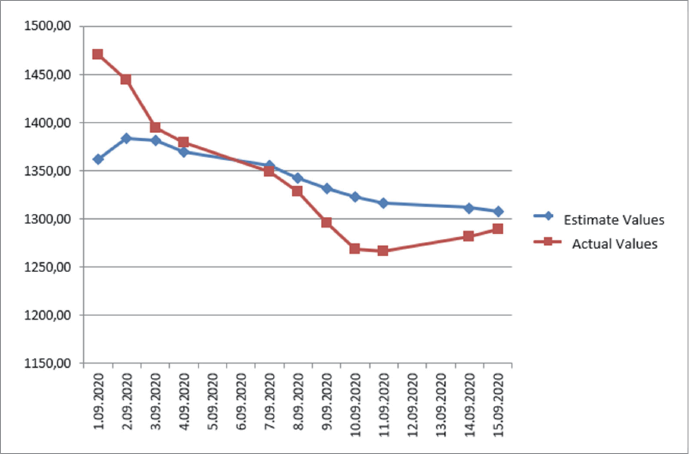
In this study, the training phase of the network was carried out with the daily data of the period 9.07.2012–31.08.2020. Due to the seasonal, nonstationary nature of the BDI and its uncertain cyclicality, it was thought that it would be more beneficial to make a short-term estimate. For this reason estimate for the period 1.09.2020–5.09.2020 was made. Since BDI is only published on weekdays, there are 11 days of data published in the first 15 days of September. Comparisons of the estimated and actual values in the 11-day period were made. In addition, performance measures were calculated. Estimated values obtained in the 11-day NARX neural network model and actual values are given for BDI in Table 4.
|
Date |
Estimate Values |
Actual Values |
|
1.09.2020 |
1362.39 |
1471.00 |
|
2.09.2020 |
1383.88 |
1445.00 |
|
3.09.2020 |
1381.44 |
1395.00 |
|
4.09.2020 |
1369.63 |
1379.25 |
|
7.09.2020 |
1355.67 |
1349.00 |
|
8.09.2020 |
1342.70 |
1328.00 |
|
9.09.2020 |
1331.76 |
1296.00 |
|
10.09.2020 |
1323.06 |
1269.00 |
|
11.09.2020 |
1316.44 |
1267.00 |
|
14.09.2020 |
1311.66 |
1282.00 |
|
15.09.2020 |
1308.40 |
1289.00 |
In Table 5, the MAPE, MAE, and RMSE performance criteria values of the 11-day estimated values are given. The value of the MAPE performance criterion was obtained as 2.96%. Therefore, since the MAPE value of the model is below 10% according to Lewis (1982), it can be said that it is in the category of “very good” models. The MAE performance criterion was calculated as 36.6 and the RMSE performance criterion as 46.68.
|
MAPE |
MAE |
RMSE |
|
2.96 |
36.60 |
46.68 |
The comparative graph of the 11-day estimated and actual values of the Baltic Dry Index with NARX neural network is given in Figure 10.
The high performance of NARX neural networks in BDI estimate is in line with the results of studies in the literature (Lin and Wang, 2014; Lin et al., 1996; Papailias et al., 2017).
Maritime transport is one of the most widely used types of transport because it is the cheapest and most reliable all over the world. Therefore, the development of maritime trade activities largely reflects the vitality of trade around the world. The reliable and independent data provider of the maritime market, the London Baltic Exchange, is a reference database for freight and derivative contracts concluded around the world. BDI data is published regularly daily. However, people who benefit from this data also need information about the level of data in the future, because the sector involves a high amount of investment and operational costs. The more information is available in the decision-making process, the easier it is to choose jobs that can have profitable results. So more information means less cost. For this reason, businesses have to shape their investment plans according to the situation of the market in the future.
The capital cost of maritime transport is quite high compared to other modes of transport. In addition, due to low profit rates, even a small amount of mobility in freight rates can cause great costs for businesses. For this reason, accurate analysis and estimating of the maritime market help businesses maximize their profits by minimizing their risks (Culliane, 1999). But with high volatility, maritime trade data is very difficult to predict. Especially with the COVID-19 epidemic, which affects the whole world, uncertainties have increased considerably. It is thought that these uncertainties will cause some permanent changes in the maritime market. Increasing technological developments and changing consumer spending habits lead to changes in globalization models and supply chains. Full-time production models come to the fore (UNCTAD, 2020).
Duru et al. (2010) estimated long-term dry cargo freight rates using Bivariate Fuzzy Time Series (BIFTS), ARIMA(2,1,3) and Holt–Winters methods. The performance of these methods was calculated using MAPE, MAE and RMSE criteria. For BIFTS, value of MAPE (%16) is value of MAE (36.62) and value of RMSE (82.41). For ARIMA(2,1,3), value of MAPE (%20) is value of MAE (50.06) and value of RMSE (99.30). For Holt–Winters, value of MAPE (%16) is value of MAE (43.85) and value of RMSE (112.24). Uyan et al. (2016) present genetic algorithm (GA) based trained Recurrent Fuzzy Neural Network (RFNN) for forecasting of long term dry cargo freight rates. For RFNN, value of MAPE (%14.96) is value of MAE (24.9) and value of RMSE (36.09). BDI has a data structure that is difficult to predict with its high volatility, uncertain cyclical structure, and seasonality. For this reason, in this study, the Baltic Dry Index was estimated with the NARX neural network. NARX neural network model, which has high performance compared to traditional methods and has never been used in the estimation of BDI, will contribute to the existing literature. Thus, for all individuals and businesses dealing with maritime trade, an estimating model is proposed that minimizes uncertainties. For the analysis, eleven independent variables were determined to be directly or indirectly related to the Baltic Dry Index. These are: Bloomberg Commodity Index (BCOM), S&P 500 Index, MSCI World Index, €/$ Parity, VIX (CBOE), US 10-Year Bond Yield (%), Brent Oil (USD/Barrel), Economic Uncertainty Index, and World Trade Volume (USD Billion), the Twitter-Based Economic Uncertainty Index (TEU) and the Twitter-Based Market Uncertainty Index (TMU). 11-day estimate results are given for the period 1.09.2020-15.09.2020 with the NARX neural networks. In order to evaluate the accuracy and effectiveness of the estimation results obtained in the study, MAPE, MAE, and RMSE performance criteria values were calculated. NARX neural network results were obtained as MAPE 2.96%, MAE 36.6% and RMSE 46.68.
As a result, this study is important in terms of proposing an estimating model that covers the early stages of the COVID-19 epidemic, which is full of uncertainties. The predictive power of the analysis has been increased with the rich variables used in the study. The difference between this study from other studies is that there no previous study could be found analyzing BDI by NARX neural network model. The difference in terms of variables is that the Twitter-Based Economic Uncertainty Index (TEU) and the Twitter-Based Market Uncertainty Index (TMU), which have not been used before in BDI estimation analysis, are included in the analysis in this study and are thought to contribute to the literature. It is thought that the estimation model proposed in the study may be useful in determining market and risk strategies for businesses and individuals interested in maritime trade, such as researchers, shipbrokers, owners, operators, traders, financiers, and charterers.
The limitation of this study is that artificial neural networks can only work with numerical data. This situation causes every explanatory variable that is effective on the dependent variable to be not included in the analysis. In addition, in this study, since the BDI data is daily, the data set consisting of explanatory variables was created from daily data. The use of daily data has made the analysis more sensitive and effective for individuals and businesses that want to use the estimated results. However, considering the overfitting feature of artificial neural networks and the daily data set, there is a short-term estimate in the study. While the use of daily data is an advantage in the study, short-term estimating can be considered as a limitation of the study. For this reason, in future studies, it is thought that making comparative studies with different data types and data frequencies by making use of different machine learning methods will enrich the literature.
Aharon, D. Y., Demir, E., Lau, C. K. M. and Zaremba, A. (2021). Twitter-Based Uncertainty and Cryptocurrency Returns. Research in International Business and Finance, 59, 1–26. https://doi.org/10.1016/j.ribaf.2021.101546.
Alon, I., Qi, M. and Sadowski, R. J. (2001). Forecasting Aggregate Retail Sales: A Comparison of Artificial Neural Networks And Traditional Methods. Journal of Retailing and Consumer Services, 8(3), 147–156. https://doi.org/10.1016/S0969-6989(00)00011-4
Baker, S. R., Bloom, N., Davis, S. J. and Renault, T. (2021). Twitter-Derived Measures of Economic Uncertainty. Technical Report. Stanford University. Palo Alto, CA.
Bakshi, G., Panayotov, G. and Skoulakis, G. (2010). The Baltic Dry Index as a Predictor of Global Stock Returns, Commodity Returns, and Global Economic Activity. In AFA 2012 Chicago Meetings Paper. (October 1, 2010).
Baltic Exchange. Access Address: https://www.balticexchange.com/en/index.html, (05.06.2021).
Barut, A., Görgün, M. R., and Erdoğdu, A. (2020). The Relationship Between Baltic Dry Cargo Index and Dow Jones Iron-Steel Index. Journal of Human and Social Sciences Research, 9(3), 3019–3033.
Basheer, I. A. and Hajmeer, M. (2000). Artificial Neural Networks: Fundamentals, Computing, Design, and Application. Journal of Microbiological Methods, 43(1), 3–31.
Bayir, F. (2006). An Application on Artificial Neural Networks and Prediction Modeling. Unpublished Master Thesis, Istanbul, Istanbul University Institute of Social Sciences.
Bildirici, M. E., Kayikci, F. and Onat, I. Ş. (2015). Baltic Dry Index as a Major Economic Policy Indicator: The Relationship with Economic Growth. Procedia-Social and Behavioral Sciences, 210, 416–424.
Bolzan, A. C., Machado R. A. F. and Piaia J. C. Z. (2008). Egg Hatchability Prediction by Multiple Linear Regression and Artificial Neural Networks, Brazilian Journal of Poultry Science, 10(2), 97–102.
Chaudhuri, T. D. and Ghosh, I. (2016). Artificial Neural Network and Time Series Modeling Based Approach to Forecasting the Exchange Rate in a Multivariate Framework, Journal of Insurance and Financial Management, 5, 92–123. https://doi.org/10.48550/arXiv.1607.02093
Chou, C. C. and Lin, K. S. (2019). A Fuzzy Neural Network Combined with Technical İndicators and its Application to Baltic Dry Index Forecasting. Journal of Marine Engineering & Technology, 18(2), 82–91. https://doi.org/10.1080/20464177.2018.1495886
Cihangir, C. K. (2018). The Impact of Global Risk Perception on Global Trade. Journal of Business and Economic Studies, 6(1), 1–10.
Cullinane, K. P. B., Mason, K. J. and Cape, M. (1999). A Comparison of Models for Forecasting the Baltic Freight İndex: Box-Jenkins Revisited. International Journal of Maritime Economics, 1(2), 15–39. https://doi.org/10.1057/ijme.1999.10
Dhamija, A. K. and Bhalla, V. K. (2010). Financial Time Series Forecasting: Comparison of Neural Networks and ARCH Models. International Research Journal of Finance and Economics, 49, 185–202.
Ding, B., Qian, H. and Zhou, J. (2018, June). Activation Functions and their Characteristics in Deep Neural Networks. In 2018 Chinese Control and Decision Conference (CCDC) (pp. 1836-1841). IEEE.
Duru, O., Bulut, E. and Yoshid, S. (2010). Bivariate Long Term Fuzzy Time Series Forecasting of Dry Cargo Freight Rates. The Asian Journal of Shipping and Logistics, 26(2), 205–223. https://doi.org/10.1016/S2092-5212(10)80002-1
Economic Policy Uncertainty. (2021). Economic Uncertainty Index. Access Address: https://www.policyuncertainty.com/EURQ_monthly.html (23.03.2021).
Economic Policy Uncertaint.y (2021). Twitter Based Market Uncertainty Index. Access Address: https://www.policyuncertainty.com/twitter_uncert.html (18.03.2021).
Economic Policy Uncertainty. (2021). Twitter-Based Economic Uncertainty Index. Access Address: https://www.policyuncertainty.com/twitter_uncert.html (18.03.2021).
Giannarakis, G., Lemonakis, C., Sormas, A. and Georganakis, C. (2017). The Effect of Baltic Dry Index, Gold, Oil and Usa Trade Balance On Dow Jones Sustainability İndex World. International Journal of Economics and Financial Issues, 7(5), 155–160.
Guzman, S. M., Paz, J. O. and Tagert, M. L. M. (2017). The Use of NARX Neural Networks to Forecast Daily Groundwater Levels. Water Resources Management, 31(5), 1591–1603. https://doi.org/10.1007/s11269-017-1598-5
Han, L., Wan, L. and Xu, Y. (2020). Can the Baltic Dry Index Predict Foreign Exchange Rates?. Finance Research Letters, 32, 101157.
Investing. (2021). Baltic Dry Index. Access Address: https://tr.investing.com/indices/baltic-dry-historical-data (18.03.2021).
Investing. (2021). Bloomberg Commodity Index. Access Address: https://tr.investing.com/indices/bloomberg-commodity-historical-data (18.03.2021).
Investing. (2021). S&P 500 Index. Access Address: https://tr.investing.com/indices/us-spx-500-historical-data (19.03.2021).
Investing. (2021). US 10-Year Bond Yield. Access Address: https://tr.investing.com/rates-bonds/u.s.-10-year-bond-yield-historical-data (18.03.2021).
Investing. (2021). VIX. Access Address: https://tr.investing.com/indices/volatility-s-p-500-historical-data?cid=1096487 (19.03.2021).
Jain, A. K., Mao, J. and Mohıuddın, K. M. (1996). Artificial Neural Networks: A Tutorial. Computer, 29(3), 31–44.
Jeong, H. M., and Park, J. H. (2017). Short-term Electric Load Forecasting in Winter and Summer Seasons using a NARX Neural Network. The Transactions of the Korean Institute of Electrical Engineers, 66(7), 1001–1006. https://doi.org/10.5370/KIEE.2017.66.7.1001
Kiracı, K. and Akan, E. (2020). Causality Relationship Between Baltic Dry Index (BDI) and Selected Macroeconomic Variables. Writings on Business and Finance – IV, 260-276.
Larose, D.T. (2005). Discovering Knowledge in Data: An Introduction to Data Mining. Vol:4, New Jersey: John Wiley and Sons Inc.
Levenberg, K. (1944). A Method for the Solution of Certain Non-Linear Problems in Least Squares. Quarterly of applied mathematics, 2(2), 164–168.
Lewis, C.D. (1982). Industrial and Business Forecasting Methods. Londra: Butterworths Publishing.
Lin, T., Horne, B. G., Tino, P. and Giles, C. L. (1996). Learning Long-Term Dependencies in NARX Recurrent Neural Networks. IEEE Transactions on Neural Networks, 7(6), 1329–1338.
Lin, Y. and Wang, C. (2014). The Dynamic Analysis of Baltic Exchange Dry İndex. In International Mathematical Forum, 9(17), 803–823.
Marquardt, D. W. (1963). An Algorithm for Least-Squares Estimation of Nonlinear Parameters. Journal of the Society for Industrial and Applied Mathematics, 11(2), 431–441.
Matrix Prime Program. (2021). Brent Oil. Access Address: https://www.matriksdata.com/website/kurumsal-urunler/matriks-prime (18.03.2021).
Mitrea, C. A., Lee, C. K. M. and Wu, Z. (2009). A Comparison Between Neural Networks and Traditional Forecasting Methods: A Case Study. International Journal of Engineering Business Management, 1(11), 67–72. https://doi.org/10.5772/6777
Papailias, F., Thomakos, D.D. and Liu, J. (2017). The Baltic Dry Index: Cyclicalities, Forecasting and Hedging Strategies. Empirical Economics, 52(1), 255–282. https://doi.org/10.1007/s00181-016-1081-9
Pham-Gia, T. and Hung, T. L. (2001). The Mean and Median Absolute Deviations. Mathematical and Computer Modelling, 34(7-8), 921–936. https://doi.org/10.1016/S0895-7177(01)00109-1
Ruan, Q., Wang, Y., Lu, X. and Qin, J. (2016). Cross-Correlations between Baltic Dry Index and Crude Oil Prices. Physica A: Statistical Mechanics and its Applications, 453, 278–289. https://doi.org/10.1016/j.physa.2016.02.018
Sahan, D., Memisoglu, R. and Baser, S. Ö. (2018). Predicting Baltic Dry Index with Leading Indicators. Dokuz Eylul University Maritime Faculty Journal, 10(2), 233–248. https://doi.org/10.18613/deudfd.495820
Sahin, B., Gurgen, S., Unver, B. and Altin, I. (2018). Forecasting the Baltic Dry Index by Using an Artificial Neural Network Approach. Turkish Journal of Electrical Engineering & Computer Sciences, 26(3), 1673–1684. https://doi.org/10.3906/elk-1706-155
Sahin, E. E. (2018). Cryptocurrency Bitcoin: Price Prediction with ARIMA and Neural Networks. Fiscaoeconomia, 2(2), 74–92.
Sarac, M., Zeren, F. and Basar, R. (2015). Interaction Between Global Gold Prices, US Supplementary Aid Spending and the Baltic Dry Index. Journal of Istanbul University Faculty of Business Administration, 44(1), 12–20.
Sert, F. (2014). Prediction of Weather with Artificial Neural Networks and Classification with Fuzzy Logic. Master Thesis, Bursa, Uludag University Institute of Social Sciences.
Siegelmann, H. T., Horne, B. G. and Giles, C. L. (1997). Computational Capabilities of Recurrent Narx Neural Networks. IEEE Transactions on Systems, Man, and Cybernetics, Part B (Cybernetics), 27(2), 208–215.
State Planning Organization, (2001). Eighth Five-Year Development Plan, Access Address: https://www.sbb.gov.tr/wp-content/uploads/2018/11/08_Gemi%C4%B0nsaSanayii.pdf, (25.05. 2021).
TCMB (2021). €/$ Parity. Access Address: https://evds2.tcmb.gov.tr/index.php?/evds/serieMarket (18.03.2021).
The Netherlands- Centraal Planbureau (CPB)- Bureau For Economic Policy Analysis (2021). World Trade Volume. Access Address: https://www.cpb.nl/en/worldtrademonitor (02.04.2021).
Trujillo, L. And Tovar, B. (2007). The European Port Industry: An Analysis of its Economic Efficiency. Maritime Economics & Logistics, 9(2), 148–171. https://doi.org/10.1057/palgrave.mel.9100177
Ucal, M. S. (2006). A Brief Review on Econometric Model Selection Criteria, C.Ü. Journal of Economics and Administrative Sciences, 7(2), 41–57.
UNCTAD. (2020). Review of Maritime Transport 2020. Shipping in Times of the Covid-19 Pandemic. Access Address: https://unctad.org/system/files/official-document/rmt2020_en.pdf. (10.06.2021).
Uyar, K., Ilhan, U. and Ilhan, A. (2016). Long Term Dry Cargo Freight Rates Forecasting by Using Recurrent Fuzzy Neural Networks. Procedia Computer Science, 102, 642–647. https://doi.org/10.1016/j.procs.2016.09.455
Wu, W., Tiwari, A. K., Gozgor, G. and Leping, H. (2021). Does Economic Policy Uncertainty Affect Cryptocurrency Markets? Evidence from Twitter-Based Uncertainty Measures. Research in International Business and Finance, 58, 1–29. https://doi.org/10.1016/j.ribaf.2021.101478
Yahoofinance. (2021). MSCI World Index. Access Address: https://finance.yahoo.com/quote/MSCI/history?period1=1195171200&period2=1616112000&interval=1d&filter=history&frequency=1d&includeAdjustedClose=true (18.03.2021).
Yang, Z. and Mehmed, E. E. (2019). Artificial Neural Networks in Freight Rate Forecasting. Maritime Economics & Logistics, 21(3), 390–414.
Yegnanarayana, B. (2009). Artificial Neural Networks. PHI Learning Pvt. Ltd.
Yilmazkuday, H. (2022). Coronavirus Disease 2019 and the Global Economy. Transport Policy, 120, 40–46. https://doi.org/10.1016/j.tranpol.2022.03.003
Yu, H., Wilamowski, B. M. (2018). Levenberg–marquardt training. In Intelligent systems (pp. 12-1). CRC Press.
Zeng, Q., Qu, C. (2014). An Approach for Baltic Dry Index Analysis Based on Empirical Mode Decomposition. Maritime Policy & Management, 41(3), 224–240. https://doi.org/10.1080/03088839.2013.839512
Zeren, F. and Kahramaner, H. (2019). Investigation of the Interaction Between Baltic Dry Freight Index and Istanbul Freight Index: An Econometric Application. Journal of International Management Educational and Economics Perspectives, 7(1), 68–79.