 (1)
(1)Ekonomika ISSN 1392-1258 eISSN 2424-6166
2023, vol. 102(2), pp. 47–67 DOI: https://doi.org/10.15388/Ekon.2023.102.2.3
Algirdas Bartkus
Faculty of Economics and Business Administration, Vilnius University, Vilnius, Lithuania.
Email: algirdas.bartkus@evaf.vu.lt
Abstract. This article presents theoretical foundations for original Phillips curve formulation and an empirical investigation, where the structure of the theoretical model serves as a template for the creation of the empirical model.
For a couple of decades the majority of empirical Phillips curve type assessments are performed using the New Keynesian Phillips curve with Calvo pricing as a benchmark for this type of relationship. New Keynesian model has solid microeconomic foundations, has proved itself very well in the analysis of price stickiness; nevertheless, it is not without limitations. The main insufficiency of New Keynesian model is that it has no direct links to the conditions and the changes that occur in the labour market. The need to encompass the conditions in labour market comes from the coincides that occur time to time when the growth rates of aggregate production may diminish or even become negative, but the level of employment may stay the same, what in turn means that the pressure on inflation won’t drop, despite the fact that production level has not increased as expected or even has decreased. This article aims to fill this gap and presents alternative theoretical foundations for Phillips curve, that lead to the model with direct links to the labour market. Theoretical foundations are necessary as they may help to minimize the risks to miss some important details or to omit important factors. Although the empirical analysis in this paper is based on Lithuanian data, it is not country specific.
Keywords: inflation; unemployment; Phillips curve; nonlinear time series models.
_________
Received: 09/11/2022. Revised: 28/03/2023. Accepted: 21/06/2023
Copyright © 2023 Algirdas Bartkus. Published by Vilnius University Press
This is an Open Access article distributed under the terms of the Creative Commons Attribution License, which permits unrestricted use, distribution, and reproduction in any medium, provided the original author and source are credited.
Phillips curve relationship and natural rate are very important concepts that help to understand how prices evolve on macro level. As mentioned in the opening sentence of the famous article “How precise are the estimates of the Natural Rate of Unemployment” by Staiger, Stock and Watson, “monetary policy in the United States often focus [...] on whether the unemployment rate is approaching its natural rate” (Staiger et al., 1997). The Phillips curve relationship for Lithuania is important for another reason, i.e. inflation. The consumer price inflation in Lithuania has a tendency to speed up and time to time to exceed all acceptable Eurozone limits. The episodes of the accelerating inflation can be observed even under high rate of unemployment. Inflation is one of the problems Lithuanian economy is facing, therefore, the identification of specific reasons is indeed vital for policy making. Also worth to keep in mind, that traditional formulation of Phillips curve implies, that dynamics of prices is a function of unemployment rate, thus it links the conditions in the labour market and the demand for labour with the firm’s pricing decisions. If labour costs play a significant role in pricing decisions, the traditional formulation may prove itself more appropriate than the currently adopted New Keynesian form.
Many empirical linear models for inflation can not be seen as sufficient models, as they simply do not pass nonlinearity or conditional heteroscedasticity tests. The careful examination of the error term of these models discloses the presence of nonlinear adjustments or heteroscedastic variance. The descriptive or stylized facts let us to assume that response of inflation on external shocks depends on the current state of the affairs in the economy, i.e. the responses of inflation on various external factors are nonlinear. These facts should be of no big surprise as the first ARCH model that was proposed by Engle dealt with the estimation of inflation equation for UK (Engle, 1982). Nonlinear behavior of this variable is well known and documented in empirical literature. Nevertheless, theoretical models are exclusively linear and do not match reality very well.
The paper is organised as follows. Section two lays out main findings in the research, that aimed to explain the dynamics of prices in Lithuania with the help of New Keynesian and traditional Phillips curves. Section three presents the theoretical foundations for the possible non-linear relationship and the main causes of it, where pricing decisions are directly linked to the labour costs and labour demand. Section four provides details on the estimation of Phillips curve relationship, using Lithuanian data. The empirical model, that is presented in fourth section, reflects the structure of the theoretical model, that was sketched and introduced in the section three. Final section contains conclusions and proposals.
In this section the terms NAIRU and natural rate will be used interchangeably as synonymouses. All empirical studies, that deal with the estimation of natural rate, can be divided in two subgroups. The first treats the natural rate as a constant, while the second sees it as a slowly changing variable. Majority of the authors, that have tried to evaluate the natural rate for Lithuanian used conventional techniques, that estimated this rate disregarding the impact of unemployment rate on the other variables of interest. Vetlov in his analysis of the determinants of growth, estimated natural rate, adopted Prior-Consistent filter (Vetlov, 2003). He used the smoothed and averaged series of unemployment rate, that were provided by Labour. According to him, the estimates of natural rate and actual unemployment level coincided for the first three quarters of 1996 and actual unemployment approached to natural rate prior 1996 and in the late 2003. The main deficiency of his study was not the reliance on Labour Office data, but the usage of filtering techniques, that produced the estimates, that had little to do with the actual events, e.g., inflation in the year 1996 was noticeably higher, compared with the rates, that were observed in the following years, when actual level of unemployment was below the threshold that what was labelled as a natural rate. The main deficiency of filtering techniques, when they are used for the estimation of natural rate, is that filters treat natural rate as a certain result of actual data, thus natural rate, that is determined in this manner, can not be considered as an adequate measure of long run unemployment level, as all variations in it are caused by short run fluctuations, that are included in the levels of actual series. This is the major reason why the estimates of natural rate and actual changes in the prices do not conform with the Phillips curve type relationship.
The one thing that all studies have in common is that the estimated natural rate for Lithuania is very high. Lithuanian branch of commercial bank Swedbank in their overview of Lithuanian economy claimed, that unemployment rate, that is close to 12 percent is also close to its natural level (The Lithuanian economy, 2013). The academic studies delivered very similar results. Constantinescu and Nguyen used the data from 2000 to 2015 and found that the average of the natural rate of unemployment was 11.2 (Constantinescu et al., 2018). Camarero, Carrion-i-Silvestre and Tamarit in their study, that deals with the estimation of NAIRUs for eight Central and Eastern European countries and Malta (Camarero et al., 2005), i.e., the countries, that accessed European Union in the year 2004, used the OLS regression approach and relied on the univariate procedure, developed by Staiger, Stock and Watson (Staiger et al., 1997). In the first step, they have determined the possible structural breaks and only then estimated NAIRUs. They have obtained shifting estimates of NAIRUs, where shifting points were determined by the results of unit root tests, specifically designed to be used for the series, that are distorted by the effects of structural breaks. Using Lithuanian data, authors found three structural breaks, the first of which occurred in May of 1995, the second in November of 1999 and the third in January of 2002. Although these dates do not coincide with any significant event, taking into account the possible lag effect, break point that occurred in May of 1995 can be attributed to the end of super-turbulent initial transition period. Second break that occurred in November of 1999 can be attributed to the Russian financial crisis, and the third break, that occurred in January of 2002 – to the membership in WTO. Once the break points were detected, authors have calculated NAIRUs, where the levels of NAIRUs were the local means of unemployment rate. The local means or the NAIRUs for Lithuania were 7.28, 10.38, 15.53 and 13.20 percent. The first drawback of this analysis is that the estimates of NAIRUs were based solely on the behaviour of unemployment rate, disregarding the effects, that unemployment rate may exhibit on the other variables of interest. The second deficiency is related to the usage of specific unit root tests. Univariate tests can not distinguish between large increases and decreases in unemployment, which are caused by the regular forces and by what is called a structural change. These tests treat all huge increases and decreases, if they occur on irregular basis, as a possible results of structural changes. The risk of wrong perception of a certain change as of a structural change is high in small samples and the time span in the analysis of Camarero, Carrion-i-Silvestre and Tamarit was only about ten years. The main motive why authors have used structural change unit root tests was that all these countries have undergone transition from socialism to capitalism. In a very broad understanding of structural change, yes these countries undergone a transition from communist-style planned economy into a market economy, but majority of the changes were introduced and implemented gradually and consistently, announcing these changes in advance. And overall, the nature of the variable, like unemployment rate, is that this variable increases at very high speed in a very short time, but declines at very small rates and during the long span of the time. This behaviour is not a sign of a structural break, this is a sign of a nonlinear adjustment during the various phases of economic cycle. Applying structural breaks unit root tests to such variable is somewhat risky, because a researcher risks that all changes in the cycle will be classified as structural breaks.
Ebeke and Everaert exploited Kalman filter for the Phillips curve type relation with core inflation that served as a proxy for the growth rate of the prices (Ebeke et al., 2014). The main advantage of their research is that they estimated natural rate, using the Phillips curve model as a reference point. The main drawback of their work was the reliance on filtering techniques, that produced the estimates of natural rate, that vary in a very narrow corridor (approximately of 2 percentage points, or in authors words “for Lithuania and Latvia, the time varying point estimate ranges between 10.75 and 13.75 percent”) and show a tendency towards a very slight decrease (historical average for the period 2002Q1:2013Q4 was 12.4 percent). The other deficiency of this study is the usage of core CPI inflation, as omission of energy and food prices, in a country where a big stake of consumption expenditures goes for the purchases of food and energy, yields a mis-perceived measure of inflation.
European Commission presents the estimates of non accelerating wage rate of unemployment, that was also on the similar high level of more than 10 percent (AMECO database), but the highest estimate, about 17 percent, of natural rate for Lithuania can be found in Dumlaos article (Dumlao, 2014). Author came to the conclusion that long run equilibrium in Lithuania does not exist or Phillips curve relationships can not be applied for the analysis of Lithuanian economy. The reason why his estimates and conclusions may be imprecise lies in the fact, that Dumlao has used very simple, almost stencil forms of Phillips equations, which had the same structure for all countries.
The main deficiencies of all the above mentioned studies is the lack of microeconomic foundations for the relationships that were estimated. The papers that are based on the New Keynesian Phillips curve do not have this shortcoming. One of the articles, that deals with this formulation and analyses Lithuanian case, was written by Furuoka (Furuoka, 2016). The author performed estimations of expectations augmented Phillips curves with labour income share, that was used as a proxy for the marginal production costs. The author estimated the equation of interest using OLS, 2SLS and GMM, and obtained the results, that in the reduced form under one estimation method implied a positive effect of marginal costs on the inflation, whereas under other – a negative. The structural estimates did not vary that strongly, but still implied very different effect of the scope. The author described all them as consistent, giving for the reader to understand that even widely varying estimates can be seen as consistent. A very similar study, also based on Calvo pricing model, was performed a little bit earlier by Virbickas (Virbickas, 2012). Dabušinskas and Kulikov conducted another similar study, that yielded similar results, to the ones obtained in the studies done by Furuoka and Virbickas. The main difference between this study and the two previous ones is that Dabušinskas and Kulikov focus on price stickiness and on how the expectations affect the development of inflation (Dabušinskas et al., 2007). All these studies focus on pricing rather than on the situation in labour market as defined in the classical formulation of the Phillips curve.
Based on the simple fact, that unemployment rate is a nonstationary variable, Marjanovic and Mihajlovic concluded that time independent natural rate does not exist and it changes with almost every change in the unemployment rate (Marjanovic et al., 2014). This conclusion follows from the knowledge that non-stationary variables do not have constant and time independent means. The authors reached their conclusion without taking into account the fact that unemployment can also be a non-linear variable, the central position measure of whom is not a mean, but an attractor towards which the variable approaches in a nonlinear way. Abbas with coauthors and Fidrimuc with Danišková have presented a good meta review of the recent developments in that kind of modelling (Abbas et al., 2016 and Fidrmuc et al., 2020).
Roeger and Herz compared traditional and New Keynesian Phillips curves, where their distinguishing feature was whether this curve was forward or backward looking (Roeger et al., 2023). This article uses the term traditional in order to emphasize the originally assumed relation with unemployment and not the output gap.
The dynamics of prices in general depends on the behaviour of buyers and sellers and on the decisions they make. Sellers choose a certain price for the good they produce in order to maximise the profits, while buyers decide what amount of goods to buy. The producers may act very straightforwardly, intending to increase the current profits or they may orientate themselves towards the maximisation of profits on the long run, sacrificing current profits for the sake of higher future profits. This option is usually based on the decisions to keep prices as low as it is possible.
Profit maximisation has to take into account three main channels how profits may be increased. The producers can raise the price, risking to decrease the quantity sold, they can decrease the price, hoping to increase the quantity sold, they can increase the overall level of output for any price level, if the aggregate demand is on the rise, they can try to reduce the production costs, leaving the prices and quantity produced as they are or changing them simultaneously as well. In all these choices, prices play a major role and even the decisions, that are related to cost reduction or increased output are also related to pricing and to the changes in price level, though price inflation equation has to be one of the characteristic equations in this theoretical macroeconomic model.
All firms are setting the prices for the products they are producing in advance. That means, that the actual behaviour of prices in period t is affected by the market conditions in period t – k, when prices for period t were set, and by expected changes of these conditions, that most probably will occur in period t. Therefore, the inflation equation has to contain certain factors that represent the actual estimates of these conditions.
Unemployment is one of the best measures of overall economic conditions, as it is an objective measure, compared with the frequently used production gap, the calculation of which requires to use various statistical filters or to apply production function, with a set of assumptions that sometimes are too restrictive. Production function and filtering approaches are too mechanic and may produce cycle estimates that do not have anything in common with actual events. Contrary to these measures, unemployment rate is the measure that is objective, does not depend on any assumption, does not require any data filtering and encompasses almost all features that are necessary to capture overall conditions in economy. If unemployment is on the rise or at a very high level, the performance of economy may be considered as poor, if it is at low level or constantly decreasing, it signals about reverse matters. The reason, why unemployment rate is a good proxy for economic conditions is that, besides giving the overall estimate of economic conditions, it allows to identify the periods in time when bargaining power of employees exceed that of employers and vice versa. Usually employees create a great deal of pressure on employers to increase the wages, when unemployment is going down or face a refusal to increase the wages when unemployment is on the rise. Wages are also related to pricing decisions, as they are the main component of labour costs and the increase in these costs may force firms to increase the prices in order to save the profits from the fall. It also may be the case, that if the firms expect the unemployment rate to be very low, they will increase the prices in advance, seeking to accumulate enough funds for further wage increases and to avoid the need to revise the prices too frequently in the future.
Selection of the functional form for the profits function Πt requires to determine how prices are set. As current prices Pt were set some time ago (for simplicity let us assume that this was done in period t – 1), taking into account the then reality, so the prices that consumers are facing in period t are in fact the expectations of the best prices for that period, based on information that was available back then, or in other words:
(1)
Multiplicative disturbance εt contains all factors, that cause the deviation of actual price from the price, that fits the above described needs of a firm at best.
Price Pt is supposed to be the average of best final prices for firms who produce various goods and set the prices for them. This price has to serve its purpose, it has to be a measure, that helps to keep profits or market share at the desired level. It is also clear that price, that is set in the end of period t – 1 for the period t, is a certain expectation of the best price, as the true best price can not be known in advance and of course the actual prices may very well change from those levels at which they were set initially. The probability that the actual price in period t, Pt will be different from that, that was supposed to be set, Et – 1(Pt*), depends very much on the frequency of the data, that is used in the analysis. In this paper the analysis is based on quarterly data and the quarter is a certain compromise frequency, as there are firms who revise the prices more frequently than once in a quarter and those who do it less, than once in a quarter. A quarter is quite a long time span and of course there exists a substantial risk that due to the effects of unforeseen changes in factors, that affect the level of production or the demand for goods, the price will be revised and the actual price Pt will be different from that, that was set in advance. The question of main importance is, what determines and what causes these changes and how price responds to the changes in factors, that determine its level.
Price serves different purposes, but the main is the maximisation of profits on the short or on the long run. Sometimes firms can sacrifice current profits for future profits, trying to increase the market share or having other priorities in mind. Therefore the analysis of possible factors, hiding under exp(εt), that summon the revision of prices, that were set a while ago, supposedly at period t – 1, should start with a profit function, specified in a manner close to the way owners, managers are perceiving and understanding the profit and the driving factors behind it. Profits Πt are the difference between the revenues and the costs. Revenues from sales depend on the quantity sold Qs,t and on the price at which these goods are sold Pt. Costs depend on the quantity produced Qp,t, on the costs per unit of production Cp,t, on the inventory in stock Qi,t and on the storage costs per unit of production Ci,t:
 (2)
(2)
Quantity produced and inventory in stock determine the level of goods supplied, while quantity sold is related to the amount of goods demanded. Here, and in the remaining equations, Qs,tPt stands for the overall turnover  where n is the number of different goods produced and sold, Pt is the average price of a basket of goods, Qs,t is a number of baskets of goods sold, so that
  . Analogously, the overall amount of production costs is
  and can be expressed as Qp,tCp,t as well, where Cp,t stands for the average costs per unit of production of a basket of goods and Qp,t is the number of baskets of goods produced, so that
  . The technical definition of the last term Qi,tCi,t is the same as of previous two and does not require any specific discussion. Although there is no direct representative agent in this models, one can easily imagine that this a producer that produces and sells the representative basket of goods. With this specification, level of prices in the equation (2) is the choice variable for the representative agent or a collective firm. Further rearrangements of equation (2) will require to redefine some of the factors, that are directly related to prices. Prices may affect profits via revenue (explicitly shown Pt factor and quantity sold Qs,t factor) and via cost (quantity produced times costs of production Qp,tCp,t) channels. Both, quantity sold and quantity produced are related to prices, both are related to demand and supply, but the first one is a bit closer to the demand and the second is a bit closer to supply. Also worth to note, that quantity produced functionally affects quantity sold.
The proper definition of turnover Qs,tPt in equation (2) has to take into the account that turnover is determined by demand and the factors behind it, like income, employment status and the prices. Here prices enter the turnover definition twice, firstly as a plain price factor, secondly, via the quantity sold Qs,t factor, which is itself a function of prices. In closed economy, the quantity demanded depends on the buying power of inhabitants. Let us assume, that total workforce Nt, consists of active and employed labour force Lt = (1 – Ut)Nt, that earns wages Wt, unemployed labour force UtNt, that is on unemployment benefits ru,tWt, and next to them there is a huge amount of old-age pensioners Np,t who receive old-age pensions rp,tWt, where ru,t and rp,t are unemployment benefits and old-age pensions replacement rates, then the turnover can be defined in this way:
 (3)
(3)
Coefficients c1, c2 and c3 denote the fractions of income that are devoted for the consumption purposes.
Definition of costs Qp,tCp,t requires to distinguish between capital, labour costs and other than labour or capital related production costs. Let us assume, that costs consist of two portions, labour and capital, where capital costs account for a certain fraction ρt of the whole capital Kt, while labour costs are related to the amount of labour hired and the wages paid. The number of workers hired Lt can be expressed as a product of the whole workforce Nt and employment rate Et, or one minus unemployment rate 1 – Ut. Other than capital or labour related production costs include the costs of raw materials and transportation, the costs of manufacture, advertisement and salesmanship costs, i.e., everything, excluding wage or capital related payments. These costs are of huge importance, when it comes to price setting, as for capital intensive industries prices of raw materials, energy and other intermediate inputs are of huger importance, compared with the level of wages, but nevertheless they will play no role in the model, as the level of prices of these inputs can not be influenced by the decisions of a particular producer virtually. Summing everything up, total costs may be written as a sum of labour, capital and material costs:
 (4)
(4)
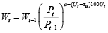
In equation (4) Cmp,t stands for the costs of materials per unit of production and the product Qp,tCmp,t is the total amount of production costs, related to the non-labour and non-capital inputs. From the right hand side variables of equation (4) wages have the closest links to the prices. Wages are very much the function of prices, as the increases in prices usually push the workers to demand the compensations for the hikes in prices from their employers and this will be the starting point for the inclusion of prices into costs equation. A simple and very frequent version of wage and price relation involves a model with a constant elasticity of wage growth rate on to the growth rate of the prices:
 (5)
(5)
Although intuitive, equation (5) does not have any practical value, as it is too simple and too far from the reality. The constancy of power a is the main deficiency in this model. If the coefficient a is equal to one, a certain relative increase in prices, causes the same relative increase in wages. If this coefficient is larger than one, wages grow at the higher rate, compared with the prices, if it is less than one, but still positive, wages grow at lower rate, compared with the prices and if it is negative, wages decline, when prices go up. Constancy of power a implies, that wages are growing on the same rate (does not matter, lower or higher, compared with the growth rate of the prices) and all short run deviations from this proportionality are totally random. Of course this is not convincing, because it is not difficult to find historical periods, when increases in prices caused much huger increases in wages, and when wages have not responded at all onto any increments in prices. That means that this elasticity cannot be constant but has to depend very much on the ongoing situation in the economy. Summing up, in a proper form, the power a on price inflation in equation (5) has to depend on the economic conditions.
The wages are of primary interest for both sides of bargains, for the workers and for the employers. The workers see the wages as the main source of well-being and the main target of their efforts, while the employers have a two-folded view on this issue. From their perspective, wages are the costs and the benefits, as higher wages result in increased outlays from the firms account, but they also tend to motivate workers, force them to work more efficiently, help to increase the loyalty to the firm and improve the psychological climate. Of course the firms want to get all these benefits with the lowest possible costs and try to delay the payment of wage increments for the workers if it is possible and of course this opportunity exists if the unemployment rate is high.
Dealing with wage setting equations one has to consider, that the effects of prices on wages depend very much on the overall economic conditions and the level of unemployment is perhaps the best measure of these conditions. When it comes to wage bargains, unemployment rate is one of the best economic characteristics, that determines by how much the wages will be raised. Under high unemployment, employers may easily reject the demands of workers for the higher wages and workers on their own may not risk to lose a job and will reconcile with a pay as it is, even if prices are growing. Completely opposite constellation occurs when unemployment is low. Summing everything up, the function for the wages paid may look like this:
 (6)
(6)
This specification is a bit different from a very popular and simple version, that is presented in equation (5). In equation (6), a represents the long run response of wage inflation on price inflation, while term (Ut – τu)100Ut encompasses all short run corrections, that are related to the unemployment level. Here τu is a very specific attractor, that defines the level of unemployment, below which wages grow at higher rate, compared with the level of prices, and above which, increases in wages only partly offset the increases in prices. Multiplication by 100 is needed for the proper scaling of the power, where both Ut and τu are proportions.
The need to define τu as a specific attractor and not as a certain average rate may be motivated in the following way. In his famous textbook “Macroeconomics”, Mankiw notes, that “natural rate of unemployment is the average rate of unemployment around which the economy fluctuates” (Mankiw, 2015). The graph that is sketched above this statement (in his book) suggests that this rate is not constant and it changes over time, responding to various structural changes, that occur time to time. Treatment of natural rate as of something that is between historical ups and downs of unemployment series may be a little misleading as it implies that wage bargaining or peculiarities of inflation suddenly change, when you are in the middle of this band. And this may not be true because this moving average is solely the characteristic of unemployment rate, while natural rate is the characteristic, that is related to the way inflation or any other variable of interest changes its rate in response to the level of unemployment, that exists. Here τu is the specific rate, that defines the turning point of the reaction of wages on prices, thus it is a certain threshold value, that marks a certain point in labour relations, above which workers start to win real increases in their wages. The power a – (Ut – τu)100Ut is the elasticity of the growth rate of wages with respect to inflation. This power is constructed intentionally so, in order to mimic the actual response of wage increases on the price increases.
Turning to capital costs ρtKt, one has to note, that capital in period t, differs from capital in period t – 1 by the amount of new investments. In the multiplicative form, this may be defined using the growth rate of capital gk,t:
 (7)
(7)
Although equation (7) is similar to a random walk, it is not. Random walk implies that gk,t has to act as a white noise, but new investments are not white noise in any way, but a function of the growth in production or of a growth in aggregate demand Mt. Preselecting aggregate demand as a reference point, capital equation may take this form:
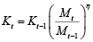 (8)
(8)
Because capital growth in equation (8) is tied to the aggregate demand and not to the production, coefficient η can be larger than unity as well. For the estimation purposes growth in aggregate demand will be proxied as growth nominal GDP as it was done by Lucas (Lucas, 1973) and Ball, Mankiw and Romer (Ball et al., 1988).
Substituting equations (3), (4) and (8) into the equation (2), we get this equation for profits:
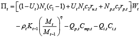 (9)
(9)
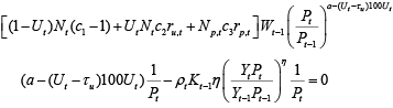
Prices enter profits equation via wage variable and via the definition of aggregate demand Mt = Yt Pt, where Yt is the real level of production. Combining equations (6) and (9) it is possible to define profits in this form:
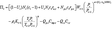 (10)
(10)
The derivative of the profit function (10) with respect to prices Pt, is:
 (11)
(11)
Multiplying both sides of derivative (11) by Pt and rearranging terms, yields:
 (12)
(12)
Despite different notation, some of the elements in equation (12) are closely related and some contain particular economic content. The real level of production Yt is very much related to the quantity sold Qs,t and the difference between these two terms is more or less random factor, thus the relationship between these factors may be expressed as:

Next term (1 – Ut)NtWt is the payroll fund in nominal terms Wf,t, which may also be defined as a product of payroll fund in real terms and prices Wrf,tPt:
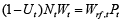
Nominal capital may be expressed as a product of real capital Kr,t and prices Pt:

With the usage of these definitions, we can rewrite the derivative (12) in this form:
 (13)
(13)
Concentrating the prices on the left side, yields the following expression:
 (14)
(14)
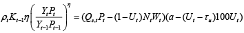
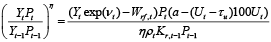
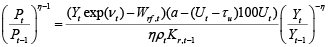
Solving equation (14) for the price inflation we obtain the final version of Phillips curve relationship:
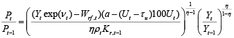 (15)
(15)
The resulting equation delivers the answer onto the question, what forces the producers to increase the price? On the one hand the increases in costs, that cannot be offset by firms decisions and on the other hand the excess demand that due to objective reasons cannot be met and if the actual growth rate mimics the changes in demand, the factor
(Yt/Yt–1)(η/(1–η)) displays exactly this feature. In equation (15) the factor(1/η)(1/(η–1)) is a specific intercept term and (Ytexp(νt) – Wrf,t)/ρtKr,t–1 is the ratio of real output minus labour costs, what is a ratio of crude real profit, related to labour to the capital costs. The higher the profits, including non-labour costs, compared to capital costs will be, the lower inflation spikes will be observed, as there would be no need to increase the prices. The effects of unemployment rate on price inflation can be traced via (a – (Ut – τu)100Ut)(1/(η–1)) factor and this effect is clearly nonlinear.
Nonlinear Phillips curves are estimated very frequently, however, these are mostly empirical studies that do not have a strong theoretical foundation. It is worth to mention the recent studies by Harding, Lindé and Trabandt or Forbes, Gagnon and Collins (Harding et al, 2023; Forbes et al, 2020), only that first study focuses on New Keynesian version, while the second on the impact of the prices of raw materials and various other inputs. This model links inflation to price setting decisions and their relationship to various factors that affect the costs of the producer. From this point of view, this article is similar to the one written by Christopher, but more universal because it does not focus solely on wages as a source of costs (Christopher, 2023).
The resulting equation (15) helps to highlight the main driving factors, that force firms to revise the prices. The first of them is the difference Ytexp(νt) – Wrf,t, which is the difference between the quantity sold and the payroll fund in real terms. The quantity sold is determined by the aggregate income, that workers earn and the payroll fund is the only source, from where the workers are paid. Hence this difference between these two real magnitudes, between the real income, which were directed into consumption and the actual payroll fund is something that is very close to unexpected income, whose source of origin is other than labour. Thus, the unexpected income tend to accelerate the prices, but their effect depends on the deviation of the unemployment from its natural rate and on the level of capital, that is available.
The second term is the elasticity of the wages on the growth rate of the prices, which is (Ut – τu)100Ut. The elasticity here is not constant and it depends on the level of unemployment and on the deviation of actual rate of unemployment from the natural rate. The more elastic wages will be, regarding the increases in prices, the more price will tend to respond with a feedback on to the changes in the economic environment. Higher elasticity and responsiveness of the wages leads to the higher responsiveness of the wages onto the unexpected income shocks, especially when actual rate of unemployment is below its natural rate Ut – τu or exceeds its natural rate by a small amount.
The third term is the capital stock. The higher capital capacities will be employed, the lower will be the need to increase the prices, responding to the various needs. This result comes from the simple fact, that in order to meet the demand, companies, that have huge capital levels, will be able to increase production quickly and without large investments.
And the fourth factor is the change in the production level. Because in this setting η can be higher than one and most probably is higher than one, the power η/(1– η) is a negative number, what in turn means that the increases in production or supply lead to the decreases in prices. The higher the η is, the closer η/(1– η) to unity is, what means that increases in demand may force the capital to grow faster. That means that if the elasticity is close to unity, forward looking producers will tend to increase production capacity with a huge certainty.
This model tells a simple story. If the prices go up, the workers start to demand a pay rise. If the production grows, when companies expect increases in demand, the companies won’t change the price at all, and will satisfy the needs of their workers. If the production goes up at the low rate, companies will also agree to the demands of the workers, only that in order to keep profits unchanged, they will raise the prices of their own goods a little bit. This increment in the prices will be small, as certain amount of it will be substituted by the effects of the increases in the production.
The producers will be inclined to increase the prices of goods, if the elasticities of the wages on the prices will be high. This means that time to time labour costs may not be covered by the increases in demand and producers will be forced to increase the prices in order to offset possible profit losses.
The inflationary response on the changes in labour market depends on the level of unemployment and on the deviation of current unemployment from its natural level, on the level of capital and on the growth rate of production. The resulting equation is nonlinear in both variables, but especially in the rate of unemployment. Possible linearisation of response function will be inevitable in the empirical part of this article.
The equations in previous section make up what can be called a theoretical model. For practical purposes the inflation function (15) has to be rearranged and put in the form, which is compatible with its economic content and with estimation possibilities. One way to simplify this function is to pick up a plausible functional form, which would allow unemployment to have a negative impact on inflation to a certain level and beyond that level, the effect would become positive. Linearization of function (15) must reflect that changes in inflation, caused by the changes in unemployment rate, are dictated by the expected conditions in labour market and by the expected increases in prices, that were observed in the near past. Possible linear forms of equation (15), may be written taking into account that the effects of the unemployment rate on the inflation depend on the income shock, on the level of capital, that is available, as well as on the unemployment rate, that existed at the moment of the effect and so on.
Inflationary expectations are a little controversial thing, as the inclusion of them into macroeconomic model requires to be very specific regarding the mathematical form of how they are formed. In macroeconomic model, inflationary expectations can be easily quantified using rational expectations hypothesis, where actual logarithmically transformed inflation πt differs from the expected rate by the random error επ,t:
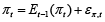 (16)
(16)
The factors that hide under expectation term are explicitly defined in function (15), while compliance with non-autocorrelation of the error term may be fulfilled by selecting a proper autoregressive approximations of inflationary behaviour. Keeping in mind that relationship in function (15) is nonlinear, the autoregressive part of the inflation may also be nonlinear.
The best fitting univariate linear model for the inflation is:
The estimates of this model are not provided here due to the fact that this equation does not play a decisive role in this article. Although the error term is unautocorrelated and is normally distributed, the squares of the residuals are autocorrelated, what in turn means that the error term is heteroscedastic or nonlinear. The simplest nonlinear univariate model for inflation can be obtained by adding the squared first lag of inflation:
 (18)
(18)
For the same reason as with equation (17), the estimates of this equation are not printed in the text. In this model the innovations and their squares are unautocorrelated, normally distributed and in all ways they act as a white noise. The second model, although formally appropriate, is not really any better than the first. The first is an autoregression with constant slopes, and the second is also an autoregression, just with a time varying first-order slope:
 (19)
(19)
First order slope in equation (17) is α1 and in equation (18) it is α1 + α11 πt–1, what in turn means that the first-order slope is time varying and it depends on the actual rate of inflation, that was observed in period t – 1. There is no other difference between the equations (17) and (18), except the one just mentioned.
Phillips curve relationship, that is presented in equation (15) contains various nonlinear interactions between the growth rate in production, the unemployment rate, investment and the income. After a little experiment it turned out that in generalized autoregressive setting the proper model for the Phillips curve relationship looks like this:
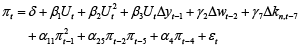 (20)
(20)
Here Δy is logarithmically transformed growth rate of real GDP, Δw is the growth rate of the wages and Δkn is the growth rate of gross fixed capital formation in nominal terms. The estimates of the coefficients of equation (20) are not presented here due to its final unimportantness. The square of unemployment is added because the scatterplot for inflation and unemployment resembles a quadratic relationship and because a similar factor to it can be found in the equation (15). Quadratic relationships have already been used by some other authors, e.g. Kochetkov has used polynomial Phillips curve relationship for Latvia (Kochetkov, 2012).
Although this equation satisfies all formal criteria, many imperfections emerged during its construction. The inclusion of the seventh lag of capital corrects the autocorrelation of the errors, but according to various indirect indications it is very likely that this lag is only spurious. Wages have a significant effect only if they are seasonally unadjusted and if they are seasonally adjusted, they are insignificant. Therefore, a more sophisticated and appropriate bilinear version was tested. The structure of bilinear model is already much closer to the Phillips curve relationship, that was described in equation (15) with the only one discrepancy from theoretical model – we found no empirical evidence that capital played at least somewhat important role in this relationship. Bilinear form for Phillips curve relationship looks like this:
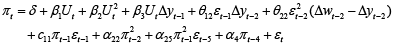 (21)
(21)
The estimates of the coefficients of equation (20) are presented in table 1.
|
Coefficients |
Estimate |
Std. Error |
t value |
p value |
|
δ |
3.2273 |
0.5228 |
6.1727 |
2.010200e-08 |
|
β1 |
-0.5754 |
0.0944 |
-6.0939 |
2.844000e-08 |
|
β2 |
0.0228 |
0.0042 |
5.4647 |
4.266600e-07 |
|
β3 |
0.0153 |
0.0017 |
9.2640 |
0.000000e+00 |
|
θ12 |
0.1188 |
0.0286 |
4.1515 |
7.613195e-05 |
|
θ22 |
0.0645 |
0.0273 |
2.3644 |
2.025687e-02 |
|
c11 |
0.2604 |
0.0482 |
5.4055 |
5.469030e-07 |
|
α22 |
0.0830 |
0.0320 |
2.5937 |
1.111987e-02 |
|
α25 |
0.0601 |
0.0229 |
2.6200 |
1.035678e-02 |
|
α4 |
0.5103 |
0.0638 |
7.9916 |
5.000000e-12 |
The resulting equation is very close to the theoretical Phillips curve equation (15) as it contains various interactions of factors that determine inflation. One of the most important factors in the formation of the growth rate of the prices is the difference between actual consumption and the payroll fund. The consumption is always associated with the income, that the employees earn. Worth to keep in mind that actual consumption may exceed that level, or may be below that level, that was associated with the planned payments to the employees. This can happen if the actual income of the employees are higher than the planned one, which were of course aligned with the production levels. Therefore, the variable that can empirically capture this difference is the difference between the growth rate of the wages and the growth rate of the real GDP. If this difference is positive, employee income growth exceeded the growth of income on the aggregate level, thus the workers have earned surplus or excess income.
The effect of unemployment on inflation can be traced out by finding the derivative of function (21), with respect to unemployment:
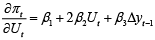
By how much the prices will change, responding to a unit change in unemployment rate depends on the exact rate of unemployment and economic growth, that were at the time of the change. If the unemployment goes up from 4 to 5 percent and the GDP in parallel declines by 2.5 percent, the rate of inflation will go down by 0.43 percentage points. If the same increase in unemployment occurs at the same level, but GDP declines by 1 percent, the rate of the inflation will go down by 0.41 percentage points and if the same increase at the same level of 4 percent occurs, only when GDP increased at 2.5 percent, the reduction in inflation rate would be only 0.35 percentage points. The responses of inflation at various levels of unemployment and for given growth rates of GDP are presented in figure 1.
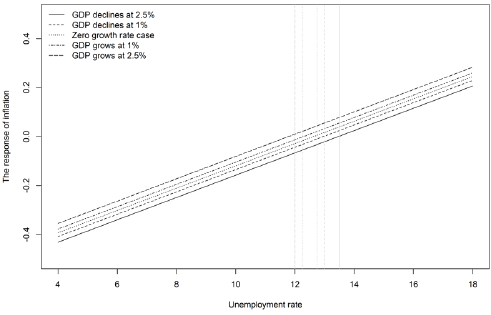
The crucial aspect here is, that the responses of the growth rate of the prices depend on the level of unemployment at which we observed these changes. One thing is when the unemployment increases by 1 percent from 5 to 6 percent and very different thing is when it increases by the same 1 percent, but from 11 to 12 percent. Overall, the higher the level at which the change will occur, the smaller the reduction in inflation will be. The greatest reductions in inflation are observed when unemployment starts to grow, and then they gradually decrease until a certain threshold is reached, beyond which inflation starts to respond positively. This change in the direction of reaction should not be a big surprise, because after initial downward corrections in the price level, inevitably the time comes when the prices have to return to normal levels, even with high rates of unemployment and with slummed demand. Excess amount of goods, that was produced prior the slump is sold, all the liabilities are covered, so it is already time for the prices to go back to normal. This is the main reason why at a high level of unemployment this dependence turns from inverse to direct. The height of this threshold is determined by the observed growth of economy in the recent past and plotted in vertical lines in figure 1. The huger is the slump in the economy, the longer the decreases in inflation rate will be observed. If the decline of economy is small, the prices tend to revert to normal quickly and if the decline is huge, they stay far away from being normal for a longer period of time. The unemployment level, which is associated with the change in the direction of response, i.e. when after long periods of deflation, we will start to meter inflation again, for different declines in GDP is from 14 to 12 percent. The supposed high natural rate of unemployment is only a point up to which the reduction in prices is observed.
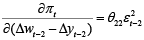
The impact of the growth rate of production on inflation can be traced out by finding the derivative of function (21), with respect to the growth rate of GDP:
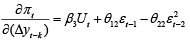
The responses of inflation at various levels of unemployment and for given growth rates of GDP are plotted in figure 2.
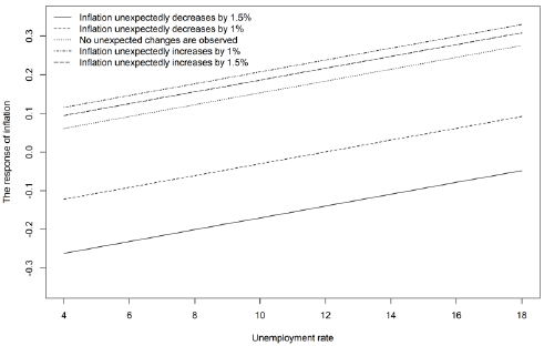
The effect of the production on the prices depends on the unemployment rate, on the unexpected changes in inflation and on their variability. If the production increases are observed when inflation unexpectedly decreases, the inflation will slow down further, only that at the low rate of unemployment this decrease will be large, whereas at the high rate of unemployment – small. If the production increases are observed when inflation unexpectedly increases, the increases in the growth rate of production will cause further increases in the growth rate of the prices, the magnitude of whom depends on the rate of unemployment that prevails. If unemployment is low, the increases in inflation will be small, but if the growth in production will be observed at the high rates of unemployment, the increment in prices will also be high. If the prices unexpectedly go up even under high rate of unemployment, that means that either the threshold where excess amount of goods was sold has been reached or the economy has to deal with excess demand or supply shocks that fuel up the prices despite the high rate of unemployment.
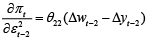
The impact of the excess income on inflation can be traced out by finding the derivative of function (21), with respect to the excess income.
The response of the growth rate of the prices onto the excess income depends on the variability of the price shocks. The higher the variance of these shocks will be, the more likely it will be that excess income will cause the increases in inflation. If the variability is equal to 1, inflation increases by 0.06 percentage point, responding to 1 percentage point increase in the excess income, but if the variability is equal to 4, inflation increases already by 0.26 percentage point, responding to 1 percentage point increase in the excess income.
The effects of the variability of the shocks on the inflation can be traced out by finding the the derivative of function (21), with respect to the variance of the innovations:
If the excess income decline by 8 percent, the rate of inflation will diminish by 0.52 percentage points, even if the variability of the shocks will increase. If the excess income declines by 2 percent, the increase in the volatility won’t cause any increase in the rate – the inflation will go down by 0.13 percentage points. The opposite effects can be observed if the excess income increase, e.g. the increase in volatility, when 6 percent increase in excess income is observed, leads to 0.39 percentage point increase in the growth rate of the prices.
The construction of the theoretical model for the Phillips curve relationship led to the following conclusions:
• Unexpected income tend to accelerate the prices, but their effect depends on the deviation of the unemployment from the natural rate and on the level of capital available.
• The more elastic wages will be, regarding the increases in prices, the more price will tend to respond with a feedback on to the changes in the economic environment.
• The higher capital capacities will be employed, the lower will be the need to increase the prices, responding to the various needs.
• The producers will be inclined to increase the prices of goods, if the elasticities of the wages on the prices will be high. This means that time to time labour costs may not be covered by the increases in demand and producers will be forced to increase the prices in order to offset possible profit losses.
The empirical analysis revealed following facts:
• The greatest reductions in inflation are observed when unemployment starts to grow, and then they gradually decrease until a certain threshold is reached, beyond which prices tend to return to their normal level.
• The height of this threshold is determined by the growth of production in the recent past. The huger is the slump in the economy, the longer the decreases in inflation rate will be observed.
• The unemployment level, which is associated with the change in the direction of response, ranges from 14 to 12 percent and depends on the actual changes in GDP.
• The effect of the production on the prices depends on the unexpected changes in inflation and on its variability. If in the recent past we have observed unexpected decreases in inflation, the inflation will go down despite that the growth rate of production accelerates. If on the contrary we have observed unexpected increases in inflation, the inflation will go up, responding to the changes in the growth rate of GDP. The low rate of unemployment can be associated with high reductions in inflation when the growth rate of the prices suddenly decreases and small increases when inflation unexpectedly increases. Whereas high unemployment supports smaller decreases in prices when they have suddenly decreased in near past and higher increases when they suddenly increased.
• The response of the growth rate of the prices onto the excess income depends on the variability of the price shocks and vice versa. The higher the variance of these shocks will be, the more likely it will be that excess income will cause the increases in inflation. If the excess income decline, the rate of inflation will diminish, even if the variability of the shocks will increase. The opposite is also true, the increase in volatility, leads to increase in the growth rate of the prices.
The performed analysis allows to propose certain recommendations on how to manage the inflation. The main precautionary signs of possible increases in the rate are: the increased variability of inflation shocks and the significant growth of excess income. If in the economy we are observing the increased variability of price shocks, the only possible reasonable response to this is the halting of the growth of excess income. This countermeasure can offset the unwanted effects of turbulent economic growth on the prices.
Syed K. Abbas, Prasad Sankar Bhattacharya and Pasquale Sgro. “The new Keynesian Phillips curve: An update on recent empirical advances.” In: International Review of Economics and Finance 43 (2016), pp. 378–403.
Laurence Ball, N. Gregory Mankiw, and David Romer. “The New Keynesian Economics and the output-inflation tradeoff.” In: Brookings Papers on Economic Activity 1 (1988), pp. 1–65.
Markus K. Brunnermeier and Christian Julliard. “Money Illusion and Housing Frenzies.” In: The Review of Financial Studies 21.1 (2008), pp. 135–180.
Mariam Camarero, Josep Lluís Carrion-i-Silvestre and Cecilio Tamarit. “Unemployment dynamics and NAIRU estimates for accession countries: A univariate approach.” In: Journal of Comparative Economics 33.3 (2005), pp. 584–603.
Malikane Christopher. “A Traditional Nominal Wage Phillips Curve: Theory and Evidence.” In: The Economic Record, The Economic Society of Australia 99(324) (2023), pp. 108–121.
Mihnea Constantinescu and Anh D. M. Nguyen. “Unemployment or credit: Which one holds the potential? Results for a small open economy with a low degree of financialization.” In: Economic Systems 42(4) (2018), pp. 649–664.
Aurelijus Dabušinskas and Dmitry Kulikov. “New Keynesian Phillips curve for Estonia, Latvia and Lithuania.” In: Working Papers of Eesti Pank, 7/2007 (2007). URL: https://haldus.eestipank.ee/sites/default/files/publication/en/WorkingPapers/2007/_wp_707.pdf
Luis F. Dumlao. “The relationship between dynamic price and dynamic unemployment: the case of the Central European-3 and the Baltic Tigers.” In: International Journal of Economic Sciences 3.2 (2014), pp. 20–42.
Christian Ebeke and Greetje Everaert. “Unemployment and Structural Unemployment in the Baltics.” In: IMF Working Paper No. 14/153 (2014). URL: https://ssrn.com/abstract=2491603
Robert F. Engle. “Autoregressive Conditional Heteroscedasticity with Estimates of the Variance of United Kingdom Inflation.” In: Econometrica, Econometric Society, vol. 50(4) (1982), pp. 987-1007.
European Commission AMECO database. URL: http://ec.europa.eu/economy_finance/ameco/user/serie/SelectSerie.cfm
Ernst Fehr and Jean-Robert Tyran. “Does Money Illusion Matter?” In: The American Economic Review 91.5 (2001), pp. 1239–1262.
Jarko Fidrmuc and Katarína Danišková. “Meta-Analysis of the New Keynesian Phillips Curve in Developed and Emerging Economies.” In: Emerging Markets Finance and Trade 56 (2020), pp. 10-31.
Kristin J. Forbes, Joseph E. Gagnon and Christopher G. Collins. “Low Inflation Bends the Phillips Curve around the World.” Working Paper Series WP20-6, Peterson Institute for International Economics, (2020). URL: https://www.piie.com/sites/default/files/documents/wp20-6.pdf
Fumitaka Furuoka. “A Scientific Inquiry on the Estimation of the Phillips Curve in the Baltic Region.” In: Engineering Economics, 27(3) (2016), pp. 276–284.
Martín Harding, Jesper Lindé and Mathias Trabandt. “Understanding PostCOVID Inflation Dynamics.” In: IMF Working Paper No. 22/10 (2023). URL: https://www.imf.org/en/Publications/WP/Issues/2023/01/20/Understanding-Post-COVID-Inflation-Dynamics-528404
Yuri Kochetkov. “Modern Model of Interconnection of Inflation and Unemployment in Latvia.” In: Engineering Economics, 23(2) (2012), pp. 117–124.
Robert E. Lucas Jr. “Some international evidence on output-inflation tradeoffs.” In: International Journal of Economic Sciences 63.3 (1973), pp. 326–334.
N. Gregory Mankiw. Macroeconomics. 9th ed. New York, NY: Worth Publishers, 2015
Gordana Marjanovic and Vladimir Mihajlovic. “Analysis of Hysteresis in Unemployment Rates with Structural Breaks: the Case of Selected European Countries.” In: Engineering Economics, 25(4) (2014), pp. 378–386.
Werner Roeger and Bernhard Herz. “Traditional versus New Keynesian Phillips Curves: Evidence from Output Effects.” In: International Journal of Central Banking, International Journal of Central Banking,8(1) (2012), pp. 87–109.
Douglas Staiger, James H. Stock, and Mark W. Watson. “How precise are estimates of the natural rate of unemployment?” In: Reducing Inflation: Motivation and Strategy. Ed. by Christina Romer and David Romer. Chicago, IL: University of Chicago Press, 1997, pp. 195–246.
The Lithuanian Economy, 2013. URL: https://www.swedbank-research.com/english/lithuanian_economy/2013/oktober/index.csp
Igor Vetlov. “Baltijos šalių ekonomikos augimo apskaita.” In: Pinigų studijos 7.3 (2003), pp. 14–34.
Ernestas Virbickas. “Estimated New Keynesian Phillips curve in Lithuania.” In: 7th International Scientific Conference “Business and Management 2012”, 10-11 May, 2012, Vilnius, Lithuania (2012), pp. 255-261.
 (17)
(17)