Ekonomika ISSN 1392-1258 eISSN 2424-6166

2023, vol. 102(2), pp. 28–46 DOI: https://doi.org/10.15388/Ekon.2023.102.2.2

Machine Learning and Data Balancing Methods for Bankruptcy Prediction

Prof. Olena Liashenko
Taras Shevchenko National University of Kyiv, Ukraine
Email: olenalyashenko@knu.ua

Assoc. prof. Tetyana Kravets
Taras Shevchenko National University of Kyiv, Ukraine
Email: tetiana.kravets@knu.ua

Yevhenii Kostovetskyi
Taras Shevchenko National University of Kyiv, Ukraine
Email: yevheniikostovetskyi@knu.ua

Abstract. The paper examines the use of various machine learning algorithms for the task of forecasting the company’s bankruptcy based on financial indicators. Different approaches to the formation of the data set on which the models are trained are compared, in particular, data balancing methods. Nine machine learning algorithms are implemented, in addition five data balancing methods (random oversampling, SMOTE, ADASYN, random undersampling, and near miss) were applied to classification tasks. It was found that bagging and random forest together with Near-Miss and Random under-sampling showed the best results in terms of the possibility of identifying bankrupt companies in small samples, while artificial neural networks and decision tree methods, together with SMOTE and random resampling, worked better on large samples. With highly unbalanced data accumulation, both small and large training samples can be used to distinguish between bankrupt companies.
Keywords: bankruptcy, bankruptcy forecasting, machine learning, data balancing, binary classification.

_________

Received: 23/12/2022. Revised: 13/04/2023. Accepted: 01/06/2023
Copyright © 2023 Olena Liashenko, Tetyana Kravets, Yevhenii Kostovetskyi. Published by Vilnius University Press
This is an Open Access article distributed under the terms of the Creative Commons Attribution License, which permits unrestricted use, distribution, and reproduction in any medium, provided the original author and source are credited.

1. Introduction

Bankruptcy is the final stage of the crisis state of an enterprise, which is characterized by the fixation of negative results of financial and economic activity, ranging from a temporary inability to fulfill monetary obligations to a full-fledged stable inability to pay debts.

The crisis of the enterprise can be caused by external and internal factors. External factors are objective to the bankrupt enterprise. They do not directly depend on the actions of the enterprise and cannot be prevented or controlled. The internal causes of bankruptcy are determined by problems within the company itself, they are subjective to the enterprise, and if they are detected in a timely manner, can be eliminated in order to avoid a crisis (Brent, 2017).

In the conditions of growing economic instability in the world, the urgency of the problem of the financial crisis is increasing both at the global and national levels, and at the level of a particular enterprise. Companies, especially small ones, always have a hard time in crisis situations and often cannot remain solvent after a crisis occurs in a company, as a result of which most of them are forced to declare themselves bankrupt.

To combat bankruptcy, it is customary to use three approaches: bankruptcy prevention, which involves the use of methods for predicting and determining the probability of bankruptcy of enterprises and timely informing management about potential threats and risks; bankruptcy warning, which consists in the introduction of anti-crisis management, controlling and economic security systems at the enterprise in order to prepare a strategy in case of bankruptcy; overcoming bankruptcy, involving the activation of all possible methods and measures to prevent the liquidation of the enterprise, the mobilization of all available forces and means through the implementation of measures aimed at bringing the economic entity out of the crisis and achieving its profitability and competitiveness.

Modern methods of crisis forecasting already make it possible to estimate the probability of a company’s bankruptcy in a few years with a fairly high accuracy. And since bankruptcy forecasting and prevention are much more effective strategies for preventing the crisis state of an enterprise than overcoming bankruptcy, enterprises need to look for ways to improve control over the financial condition of an enterprise and determine the probability of bankruptcy, since each individual enterprise is exposed to the risk of external influences or internal factors that can lead to the insolvency of the company.

In the conditions of the current level of uncertainty in the economy, an important task for enterprises is to choose the best models for predicting bankruptcy. Classical methods of financial analysis and economic-mathematical modeling have proven their high ability to predict bankruptcy. However, at the current level of technology development, preference is given to computer models due to their higher efficiency and accuracy.

After a series of global economic crises with serious consequences for the US economy, there is a trend towards a constant increase in the number of US companies declaring bankruptcy. This is due to the fact that US financial institutions have established bankruptcy procedures that satisfy both the debt restructuring needs of the debtor and the financial interests of creditors (Senbet et al., 2012).

Given the latest research in the field of US bankruptcy, it can be concluded that over the past decade there has been a constant increase in the number of bankrupt companies in the US. Especially in 2020, due to the COVID-19 pandemic, the number of US companies filing for bankruptcy peaked from the crisis in 2008-2009, and the number of companies with assets of more than one billion dollars that filed for bankruptcy became the largest in the US since 2005. In the first half of 2021, the number of bankruptcies of private and public American companies exceeded the average for these indicators for the period from 2005 to 2020 (Schwartz et al., 2021).

One of the biggest problems when filing for bankruptcy in the US is the relatively high cost of the procedure, which prevents approximately 25% of companies from making all the necessary payments to complete the procedure. This results in either a significant delay in filing or another type of bankruptcy filing, which cumulatively puts the company at an even greater disadvantage (Litwin, 2020). Thus, despite certain advantages of filing for bankruptcy, insolvency status strongly affects the company’s operations, investment attractiveness and credit scoring, which leads to further financial problems in the company, the loss of investors and the inability to find new ones. Therefore, in the context of constant economic instability in the world and a constant increase in the number of bankruptcies in the United States, companies, and especially American ones, need to introduce methods of financial monitoring and bankruptcy forecasting.

The purpose of this paper is to compare the predictive capabilities of various machine learning algorithms for predicting the bankruptcy of an enterprise in the case of a highly unbalanced data set. To achieve this goal, the following tasks were set: to determine the features of bankruptcy forecasting using machine learning methods; analyze various machine learning algorithms for bankrupt classification problems; apply data balancing methods; choose a system of indicators to assess the accuracy of classification; compare machine learning algorithms and data balancing methods based on selected accuracy metrics. The object of the study is the bankruptcy of enterprises, and the subject is modeling the interdependence between bankruptcy and a set of indicators of the company’s financial performance. The research methods are 9 machine learning algorithms (bootstrap aggregation, support vector machines with linear and radial basis kernel, artificial neural networks, random forest, boosting algorithm, k-nearest neighbors’ algorithm, decision trees and logistic regression), as well as 5 balancing methods data (Random over-sampling, SMOTE, ADASYN, Random under-sampling and Near-Miss).

The practical value of the work lies in the fact that the materials and models of the study can be used by enterprises to analyze the current financial situation and determine the likelihood of a company’s bankruptcy.

The article is structured as follows. After the introduction, Section 2 presents an analysis of recent research. Section 3 presents the methodology used, describing machine learning algorithms, as well as data balancing methods. Section 4 shows the results of a study of applying the technique to the data of American companies that have officially declared themselves bankrupt. Finally, Section 5 presents the main findings.

2. Literature Review

When building models and prognosticating bankruptcy in this paper, we used the approaches of both static models described in classical investigations and more modern intelligent methods for predicting bankruptcy. We can distinguish the following classical approaches used in this research: multiplicative discriminant analysis, which measures the risk of bankruptcy of each company with a high degree of accuracy; Altman’s Z-model by adding various financial indicators, the accounting of which increased the accuracy of bankruptcy forecasting; approach to classification based on bootstrap samples; random forest algorithm; support vector machines.

Of the contemporary investigations, this article was influenced in particular by the paper of F. Barbosa, H. Kimura and E. Altman (2017), which describes the use of various machine learning algorithms for bankruptcy prediction based on data from more than 10,000 North American companies. The research is based on a comparison of modern intellectual methods for predicting bankruptcy with statistical methods, in particular, with Altman’s discriminant analysis. As a result of this study, the authors managed to increase the accuracy of model predictions by an average of 10% compared to traditional methods, and also justify the use of additional factors for model training.

A systematic review of bankruptcy prediction models is proposed by Alaka et al. (2018). This study shows how eight popular and promising tools work based on 13 key criteria in the field of bankruptcy predictive model research. These tools include two statistical tools: multiple discriminant analysis and logistic regression; and six artificial intelligence tools: artificial neural network, support vector machines, approximate sets, case-based reasoning, decision tree, and genetic algorithm.

Y. Shi and X. Li (2019) review the literature on corporate bankruptcy prediction models based on the existing international academic literature in the field. It was established that the two most commonly used and studied models in the field of bankruptcy forecasting are logistic regression (logit) and neural network. Recently, however, many other innovative methods have been applied in this field, such as machine learning models, owing to new computer science and artificial intelligence technologies.

The article by Y. Qu, P. Quan, M. Lei, Y. Shi (2019) describes the most well-known machine learning and deep learning approaches for classifying bankrupt companies, and also systematizes the results of various studies on the use of these methods for predicting bankruptcy. The authors touch upon the topic of possible changes in bankruptcy forecasting methods and possible future trends in this direction.

S. Mehtab and J. Sen in their study (2020) compare different machine and deep learning algorithms for stock price prediction, and also differentiate the application of classification and regression models, using and describing a large number of model accuracy measures.

Machine learning methods are used to solve various economic problems. For example, research (Geldiev et al. 2018) focuses on applying machine learning to build an accurate predictive model; debt management is assessed using support vector machines (Zakhariyev et al., 2020), consumer behavior of food retail chains is clustered using machine learning algorithms (Lyashenko et al., 2021); house prices in Bulgaria are projected using time series models (Iliychovski et al., 2022).

The article by R. Brenes, A. Johanssen and N. Chukhrova (2022) presents for the first time a comprehensive literature review on the topic of statistical and intelligent models for predicting the bankruptcy of firms. The authors study the discriminatory ability of the multilayer perceptron (MLP) in the context of bankruptcy prediction. The case study is based on a dataset of Taiwanese firms and includes a comprehensive comparative analysis.

I. Miroshnichenko and V. Krupin (2022) explore the feasibility of using machine learning algorithms to assess the probability of bankruptcy up to 1 to 5 years using the example of companies that went bankrupt in 2000-2012 and non-bankrupt companies in 2007-2013. As a result of the study, the accuracy of predicting bankruptcy on average at the level of 77% was obtained and ways to improve the models were proposed, including balancing classes in the training sample, analyzing the influence of each of the predictors on the classification results, using qualitative indicators along with quantitative ones, as well as using ensemble and deep learning models.

The uniqueness of this work in comparison with those described above lies in the comparison not only of machine learning models, but also of different approaches to the formation of a training sample. It was investigated how the balancing of data in the training sample affects the accuracy of the classification results. As a result, it was revealed which models are most capable of predicting bankruptcy, as well as which approach to the formation of a training sample provides the highest prediction accuracy.

3. Methodology

Machine learning is a subset of artificial intelligence, a set of algorithms and statistical tools used to “teach” computers from their own experience to incrementally improve their performance. Machines are trained on large arrays of input data, finding certain patterns, which makes it possible to predict the future behavior of models. One of the most widely used approaches to the application of machine learning methodology is classification problems, in which certain properties inherent in classes are evaluated and the characteristics that distinguish a particular observation from other classes are identified. During the learning process, the machine assigns observations to one class or another based on certain characteristics.

This paper compares the use of the following machine learning approaches to classify bankrupt companies: bootstrap aggregation, support vector machines, artificial neural networks, random forest algorithm, boosting algorithm, k-nearest neighbors, decision tree algorithm, and logistic regression.

Bootstrap aggregation, bagging (Mehtab et al., 2020)

Bootstrap aggregation refers to the so-called ensemble learning methods, which use a combination of several methods to achieve a more accurate prediction result. This algorithm is based on a bootstrap that generates random samples with substitutions from a given training set. Independent classifications are then performed on each resulting data subset, and then the results are pooled using the model averaging method, which reduces model overfitting and inaccuracy.

Support Vector Machines (Horak et al., 2020)

An optimization model built with support vector machines is based on the transformation of one mathematical function by another function, called the “kernel”, and serves to determine the largest distance between the most similar observations belonging to different classes.

The “kernel” converts the original data into multidimensional ones. After that, it is necessary to find the hyperplane with the largest distance between classes in space. New data is plotted in the same space and a prediction is made as to whether it belongs to a class based on which side it falls on.

The “kernel” can be a linear or non-linear function. The former is mainly applied when the data is linearly separated. In reality, data, especially economic ones, is very rarely completely separable, and therefore the linear kernel function does not provide high prediction and classification accuracy due to the complexity of empirical data analysis. The support vector machine then allows the use of the error section and non-linear kernel functions (Barboza et al., 2017).

Artificial neural networks (Silva et al., 2017)

Artificial neural networks are one of the most widely used approaches in machine learning that mimic the neurons of the human brain. The network consists of nodes and links between them, which are located at several levels. The first level is the input and the last level is the output resulting from the classification; in addition, the network may have one or more intermediate hidden layers.

Random Forest (Sadorsky, 2021)

Random Forest is another ensemble learning technique whose main idea is to improve the classification capabilities of bootstrap aggregation by reducing the correlation between each component in the final ensemble and reducing model overfitting during the training phase. This is achieved by introducing additional randomness in the construction of the final model.

Boosting (Qu et al., 2019)

Boosting is a technique that first derives a base classifier from an initial dataset, then adjusts the distribution of the training dataset based on the output of the base classifier, and trains the next base classifier with the adjusted sample distribution.

Unlike the initial aggregation, in the final classification the classifiers are not equal, and the number of votes for each class is calculated taking into account the final weights of the voted classifiers.

K-nearest neighbors (Makridakis et al., 2018)

The k nearest neighbor method is a non-parametric learning-by-example algorithm that makes predictions by comparing new data with the most similar data in the training set. To do this, the Euclidean distance between the test observation point and all points of the training sample is calculated.

Decision Tree (Cho et al. 2010)

The algorithm creates strictly binary decision trees, so that each node has exactly two branches. The algorithm recursively splits the observations in the training dataset into subsets of records with similar target attribute values. The trees are built by exhaustively searching at each node for all available variables and all possible split values, and choosing the optimal split based on some criteria of “correct split”.

Logit regression (Subasi, 2020)

Logistic regression is a linear model that uses a sigmoid plot to perform classification. Due to this, the model allows you to get a result in the interval [0; 1], which facilitates the possibility of probabilistic interpretation of the results, showing the probability of belonging to a class.

Since most machine learning algorithms assume that the training set is balanced by default, these models do not take into account the distribution of classes in the training set. The results are often unsatisfactory and deviate from the class distribution of the majority of the sample, this is due to the fact that any classification algorithm tends to minimize the overall classification error. And since the contribution of the minority class is very small, the algorithms become more biased towards the majority class. In other words, this happens because the algorithm does not get the necessary information about instances of the smaller class to make an accurate prediction.

In this study, the following training sample balancing methods are used:

• Random oversampling is a data replication technique meaning random duplication of minority items (Brownley, 2021).

• Synthetic Minority Resampling Technique (SMOTE) is the artificial creation of new minority class elements based on k nearest neighbors (Veganzones et al., 2018).

• The Adaptive Synthetic Sampling (ADASYN) approach, which is a complement to SMOTE and means generating more synthetic data for minority examples that are harder to learn from than minority examples that are easier to learn from.

• Random undersampling, in which a certain number of majority class observations are removed from the data set to achieve class equality (Pykes, 2022).

• Near-Miss is the removal of elements of the majority class that are closest to a certain number of elements of the minority class (Mqadi et al., 2021).

The following indicators were used to compare models (Liang et al., 2016).

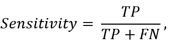
Sensitivity refers to the ability of the classifier to detect all positive data samples (i.e., non-bankrupts). It is calculated according to the formula:

(1)

where TP (true positives) are correctly classified non-bankrupts, FN (false negatives) are non-bankrupts classified as bankrupts.

Type I error is calculated based on Sensitivity:

(2)

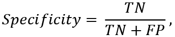
Specificity is a measure that shows the probability, that a bankrupt company will be classified exactly as bankrupt. It is calculated according to the formula:

(3)

where TN (true negatives) are correctly classified bankrupts, FP (false positives) are bankrupts, classified as non-bankrupts.

Type II Error is determined as:

(4)

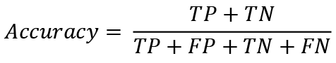
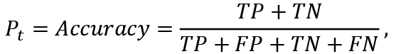
Accuracy is the proportion of positive and negative observations that were correctly classified. Mathematically calculated as:

(5)

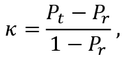
Cohen’s kappa coefficient (κ) is a statistic used to evaluate the reliability between the results of a classifier and the real situation or two classifiers. Unlike the measures described above, kappa takes into account the possibility of a random match between two classifiers. It is calculated according to the formula:

(6)

where P_t is the proportion of correctly classified observations, that is the accuracy of the classification, therefore:

(7)

and P_r is the proportion of random transactions, which were guessed by the models by chance. It is calculated as follows:

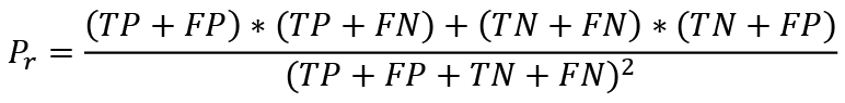(8)

The value of the Cohen’s Kappa coefficient can vary from -1 to 1, but is most often in the range from 0 to 1, where 1 means a completely correct classification, 0 means that the classification results are no better than a simple random guess. A negative value indicates that the results are worse than random guessing, but this situation is extremely rare.

The positive predictive value (PPV) measures the proportion of true positive observations among all examples classified as positive. Thus, PPV means the accuracy of classifying data as “non-bankruptcy”. The calculation is carried out as follows:

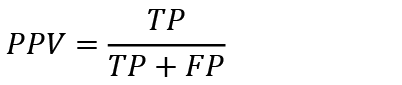(9)

The PPV is related to the false discovery rate (FDR), which is equal to:

(10)

Negative predictive value (NPV) is the opposite of PPV and represents the proportion of true negative observations among ones, that were classified as bankrupt. It is calculated according to the formula:

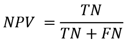(11)

Similarly, NPV has a corresponding measure – the false omission rate (FOR), which is equal to:

(12)

The F₁ measure is used when the test data set is highly imbalanced and the non-bankrupt cases significantly exceed the target cases. In this case, Sensitivity turns out to be very poor even with very high classification accuracy.

The F₁ measure takes into account the harmonic weighted average of PPV and Sensitivity. It is calculated according to the formula:

(13)

The receiver operating characteristic curve (ROC curve) or error curve is a graph that allows you to evaluate the quality of a classification by visually depicting the true positive rate ratio (TPR), which is equal to Sensitivity, and the false positive rate (FPR), that is, the proportion of bankrupts that were classified incorrectly, equal to:

(14)

This graph shows the ratio of these indicators for each threshold value.

AUC is simply the area under the ROC curve, which indicates the probability that a classifier will rate a randomly selected positive observation higher than a randomly selected negative observation. In other words, AUC is a measure of separation, which means the ability of a classifier to distinguish between the distribution of sample classes. The closer the AUC is to 1, the better the classifier is able to differentiate between minority and majority sample classes. When working with unbalanced data, this indicator is better than classification accuracy. To calculate the AUC, one must use the formula:

(15)

4. Research Results

Part of the dataset downloaded from kaggle.com (Sanyal, 2021) was used to study company failures. The database contains data on the financial performance and bankruptcies of US companies from 1980 to 2017, however, since 2014, there are no bankruptcies in the data. Therefore, the models were built on the basis of data from US companies that officially declared bankruptcy between 1980 and 2014 and for which financial information is available for at least two years before filing bankruptcy, as well as companies that did not go bankrupt during this period.

Thus, a period was taken in which it was possible to compare bankrupts and non-bankrupts. Since the work was not intended to teach the model to make a forecast for the current years, but only to conduct a comparative analysis of machine learning algorithms, it was not so important to have the most up-to-date data for these purposes.

The raw dataset included some observations where several variables were empty. To improve the performance of the models in the future, these observations were excluded from the dataset. Thus, 3,823 non-bankrupts and 14 bankrupts were excluded from the data.

The final set consists of 69,290 observations of companies, of which 557 are bankrupt and 68,733 did not declare bankruptcy during the specified period. The distribution of bankrupt and non-bankrupt companies is shown in fig. 1-2.

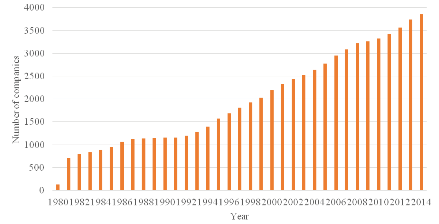
Fig. 1. Total number of observations, by year from 1980 to 2014

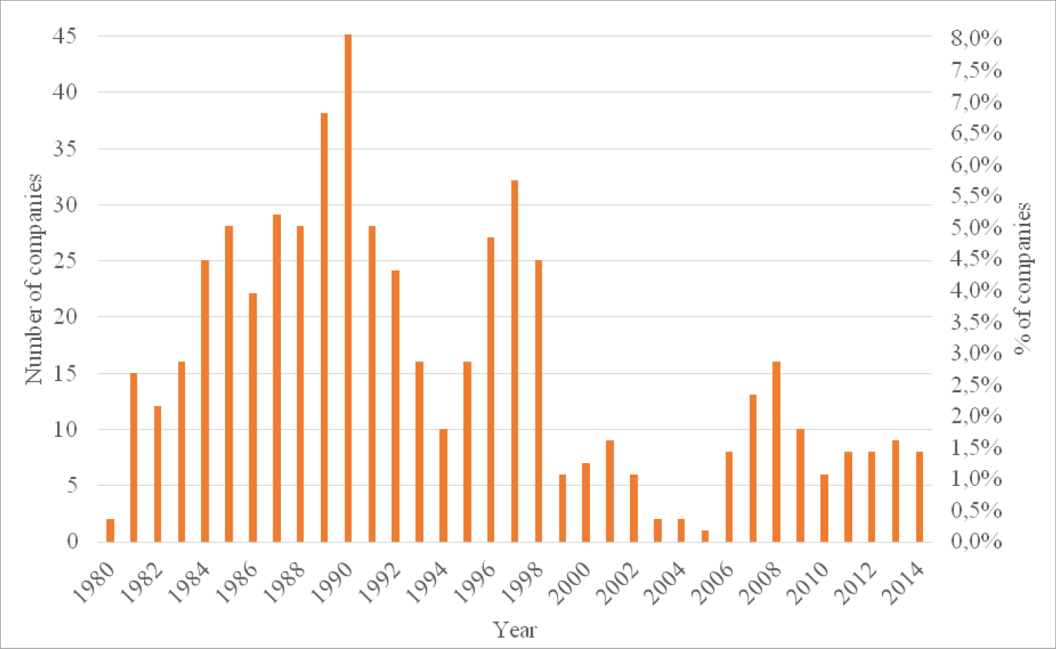
Fig. 2. Distribution of bankrupt companies by year from 1980 to 2014

On fig. 1-2 it can be seen that although the number of observations increases every year throughout the entire period, the main part of bankrupt companies falls on 1980-2000.

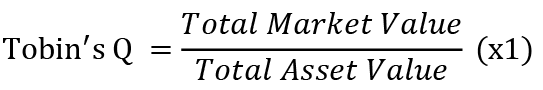
The uploaded data included a set of 13 financial indicators. These variables represent different aspects of the financial soundness of companies. The first two variables in the data are:

•

•

The following five variables were taken from the Altman’ss model, which was one of the first to predict the bankruptcy of a company:

•

•

•

•

•

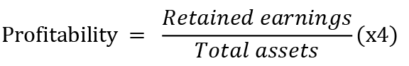
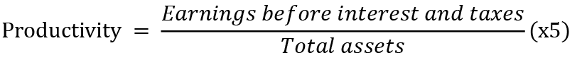
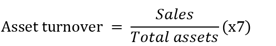
Also, the data set includes among the variables other indicators of the company’s financial results:

•

•

•

•

•

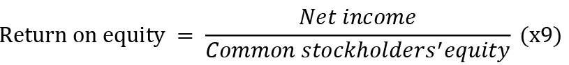
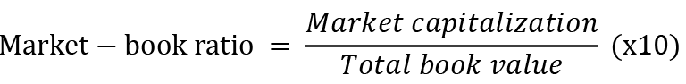
• Number of employees growth/decline ratio =

Based on the statistical indicators given in tables 1-2, it is possible to compare the structure of the groups of bankrupts and non-bankrupts. Thus, the values of each variable on average between bankrupts and non-bankrupts do not differ significantly, with the exception of x2, x9 and x10, which can serve as some indicator that the company is bankrupt. In general, the range of each of the variables vary significantly in the two groups and is significantly smaller for bankrupts, which can be explained both by a smaller number of observations and more stable values of financial indicators for bankrupt companies, which is also confirmed by a much lower variance and standard deviation of the bankrupt group.

As can be seen from Tables 1 and 2, the ranges of variables diverge greatly from each other, which can lead to poor accuracy of the constructed models. That is why data normalization was used before building models. After this process, all variables are set in the range from 0 to 1.

Table 1. Statistical indicators of variables by groups of bankrupts or non-bankrupts for variables x1-x7

		x1	x2	x3	x4	x5	x6	x7
Range	Bankrupts	226,92	142458,5	174,24	1008,28	72,59	623,63	15,97
	Non-bankrupts	25969,2	439339,0	25969,5	26238,1	1276,92	83781,3	277,8
Mean	Bankrupts	3,23	-218,18	-0,77	-8,20	-0,60	0,86	1,47
	Non-bankrupts	4,99	-17,34	-0,98	-8,74	-0,22	1,65	1,16
Variance	Bankrupts	163,17	30255294,9	63,27	3905,35	11,91	542,63	1,80
	Non-bankrupts	17214,1	6242031,7	11227,2	75491,1	43,61	86426,2	5,37
Standard error	Bankrupts	0,54	233,06	0,34	2,65	0,15	0,99	0,06
	Non-bankrupts	0,50	9,53	0,40	1,05	0,03	1,12	0,01

Table 2. Statistical indicators of variables by groups of bankrupts or non-bankrupts for x8-x13

		x8	x9	x10	x11	x12	x13
Range	Bankrupts	812,29	8095,20	10026,64	15,93	357,79	128,00
	Non-bankrupts	30570,2	100103,9	1667828,3	14232,0	39877,4	2700,00
Mean	Bankrupts	-3,50	-27,44	68,22	0,02	1,49	0,58
	Non-bankrupts	-6,32	-2,67	481,63	1,07	2,16	0,32
Variance	Bankrupts	1391,00	130202,68	315129,91	1,38	331,19	48,71
	Non-bankrupts	35748,9	140507,52	64416999,6	4815,39	39340,3	186,36
Standard error	Bankrupts	1,58	15,29	23,79	0,05	0,77	0,30
	Non-bankrupts	0,72	1,43	30,61	0,26	0,76	0,05

Table 3 shows the correlation matrix between some variables. The x3 indicator - liquidity, is most correlated with other variables, namely, Tobin’s quality factor, profitability and return on equity, which is explained by the fact that liquidity is calculated using net working capital and total assets, which are also taken into account in the above indicators. Tobin Q also has a high inverse correlation with profitability and return on equity. All other variables have a low correlation with an average of 0.0016.

Table 3. Matrix of variables with the highest correlation

	x1	x3	x4	x9
x1	1	-0,85	-0,5718	-0,6801
x3	-0,85	1	0,6036	0,8423
x4	-0,5718	0,6036	1	0,3263
x9	-0,6801	0,8423	0,3263	1

For machine learning algorithms, the data was divided into training and test sets in two ways. The first way is that the training sample is chosen much smaller than the test sample, as in Altman’s work. This is done, firstly, so that the training data is balanced, and, secondly, it is believed that with a large set of tests, it is possible to more accurately evaluate the results of model training (Malato, 2020).

For machine learning algorithms, the data was divided into training and test sets in two ways. The first way is that the training sample is chosen much smaller than the test one. This is done so that the training data is balanced, because with a large set of tests, you can more accurately evaluate the results of model training. For this approach, the data was split into 80% training set and 20% test set. Then, all bankrupt companies were selected from the training sample (451), and the same number of bankrupt companies were randomly selected from the same sample. All other observations from the two samples were assigned to the test data set. Thus, a balanced training set of 902 observations and a test set of 68,388 observations were obtained.

The second approach is to split the original data into two sets: 80% of the data for training and 20% for testing. However, since with this approach the training sample turned out to be very unbalanced (451 bankrupt and 54,981 non-bankrupt), the following data balancing methods were applied to it: the “bankruptcy” and 54,981 “non-bankrupt” - bankrupt” classes; SMOTE - a set of 54,571 observations of the “bankruptcy” class and 54,981 “non-bankruptcy” class observations was received; ADASYN is a set of 54,843 bankruptcies. received class “bankruptcy” and 54981 class “non-bankruptcy”; random undersampling - a set of 451 observations of the “bankruptcy” class and 451 “non-bankruptcy” classes was obtained; Near-Miss - a set of 451 observations of the bankrupt class and 451 observations of the non-bankrupt class. The test sample size in each case of training data balancing was 13,858 observations.

Prior to building the models, the hyperparameters were tuned as follows. Hyperparameters and their respective intervals were chosen. After that, models were built with all possible combinations of hyperparameters and errors were estimated. For the final models, combinations of hyperparameters with minimal error were selected. As a result, the following hyperparameters were established:

• Class threshold for each model – 0.5;

• Number of bootstrap replicants for the Bagging algorithm – 25;

• Number of hidden layers for Artificial Neural Networks - 30;

• The number of trees for the Random Forest algorithm is 500.

In addition, several hyperparameters were constant and not tuned, this is due to the fact that there are generally accepted methods of setting parameters. This is the number of variables chosen at random as candidates for each split in the random forest algorithm, which were established to the smallest integer greater than the square root of the number of independent variables. And also, the number of neighbors for the KNN algorithm, which was assigned the value of the smallest integer greater than the square root of the train sample length.

The essence of evaluating the results of classification carried out using machine learning is that the accuracy of classifying test data by a model trained on a training set is estimated using certain metrics.

The following model designations are used hereafter: bootstrap aggregation - Bag, support vector machines with a linear kernel function - SVML, support vector machines with a radial kernel function - SVMR, artificial neural networks - ANN, random forest - RanFor, boosting - Boost, k- nearest neighbors - KNN, decision trees - DecTree, logistic regression - Logit.

For ease of comparison, table 4 shows the average scores for the training data options for each of the models, and table 5 compares the results based on the average scores of the models for each of the models. methods.

All balancing models and algorithms were evaluated on several metrics such as sensitivity, specificity, AUC, accuracy, Cohen’s kappa, PPV, NPV, and F1-Score. The greatest attention in estimating the results was paid to Sensitivity to control for the error of the first kind associated with the incorrect assignment of bankrupts to the class of non-bankrupts; Specificity for type II error control, which means classification of non-bankrupts as bankrupts; AUC as a good metric for analyzing how models can separate data from different classes. The other metrics were more of an additional check if the primary metrics chosen did not give a clear result which model was better.

Table 4. Average assessments of the adequacy of the classification results of each of the models

Model	Sensitivity	Specificity	AUC	Accuracy	κ	PPV	NPV	F1
Bag	90,99%	59,28%	75,13%	90,75%	9,90%	99,69%	6,90%	95,01%
SVML	80,22%	57,86%	69,04%	80,06%	2,87%	99,66%	2,14%	88,78%
SVMR	80,07%	64,62%	72,34%	79,96%	3,14%	99,71%	2,28%	88,72%
ANN	81,97%	74,69%	78,33%	81,92%	4,41%	99,79%	2,94%	89,95%
RanFor	91,90%	53,30%	72,45%	91,61%	9,93%	99,65%	13,56%	95,47%
Boost	78,14%	62,58%	70,36%	78,02%	2,17%	99,65%	1,77%	87,54%
KNN	59,66%	65,09%	62,38%	59,72%	1,65%	99,51%	1,52%	71,22%
DecTree	81,44%	78,14%	79,79%	81,43%	4,03%	99,83%	2,73%	89,66%
Logit	65,63%	61,16%	63,40%	65,60%	1,60%	99,61%	1,58%	73,99%

As a result of training models on various training data sets and classifications of bankrupt companies, the following conclusions can be drawn. Thus, the approach to choosing data for training models in most cases had a significant impact on which models will perform better in the classification of bankrupt companies.

Table 5. Average measures of adequacy for each method of training set formation

Training set formation method	Sensitivity	Specificity	AUC	Accuracy	κ	PPV	NPV	F1
Balanced training set	80,51%	71,91%	76,21%	80,49%	0,96%	99,94%	0,64%	89,06%
Random over-sampling	81,90%	47,69%	64,79%	81,63%	5,35%	99,49%	8,54%	87,87%
SMOTE	75,00%	61,43%	68,21%	74,89%	6,09%	99,60%	4,41%	81,56%
ADASYN	82,59%	58,39%	70,49%	82,41%	6,28%	99,61%	4,49%	89,94%
Near-miss	79,96%	73,27%	76,52%	79,91%	4,25%	99,74%	2,95%	88,67%
Random under-sampling	73,38%	71,80%	72,59%	73,37%	3,54%	99,68%	2,58%	83,14%

However, those models were also found, the effectiveness of which practically did not depend on the training set. For example, SVML performed the worst in every case. The algorithms of the decision tree and artificial neural networks showed satisfactory results in the form of accuracy on average 81.43% and 81.92%, respectively, and specificity on average 78.14% and 74.69%, respectively, which is the best according to table 4. result among models by the percentage of correctly classified bankrupt companies. Also, SVMR always had good results in classification accuracy, sensitivity, and F1, but specificity always was low, so this model is not able to correctly classify most of the bankrupts.

As for other models, their results varied greatly depending on the training set. For example, algorithms using decision trees, namely bootstrap aggregation and random forest, gave the best classification results whenever the training set was significantly smaller than the test set (i.e., near-miss methods were also applied to the training set). At the same time, data reproduction methods gave lower results in the classification of test data. For instance, the models failed to classify the majority of bankrupts as bankrupts (although the training efficiency of these models was high). Such results can be explained, firstly, by the shortcomings of data reproduction methods: the formation of data samples that are far from real, overfitting problems, etc. Secondly, classification problems can be caused by shortcomings of the models themselves, for example, an incorrectly selected number of bootstraps for bagging.

The boosting algorithm together with KNN also showed the best results with a small amount of training data, in particular with an initially balanced set, and when using data augmentation methods, the results of the classification accuracy of the Boost algorithm dropped to 65 -75%, and KNN when training on large sets generally showed one of the worst results among all models.

Logistic regression had an extremely low adequacy of the classification results when multiplying training data using the Random oversampling and SMOTE methods, and with all other approaches to choosing a training sample, its results were average (at the level of approximately 75% of correctly classified observations).

Taking into account the average estimates presented in table 5, it can be argued that training models based on training data, the size of which is small and much smaller than the test sample, i.e. with an initially balanced sample, as well as with the application of the Near-Miss and Random undersampling methods, it gives a better classification and, in particular, the identification results of the “bankruptcy” class. And data augmentation methods, although they have higher sensitivity and accuracy, erroneously classify a significant number of bankrupt companies as “non-bankrupt”, which is less effective in practice.

In general, as a result of these calculations, it can be concluded that the best data generation method for model training in the context of this particular study is either a balanced set approach from the beginning, in which we have higher Accuracy and sensitivity, but slightly lower specificity or a “near miss” approach, in which models have slightly lower accuracy and sensitivity on average, but classify more bankrupts as bankrupts.

5. Conclusions and Discussion

Constant monitoring of the financial condition of the company is extremely important to identify signs of future bankruptcy, therefore, the management of any company is constantly faced with the task of finding a bankruptcy forecasting method that would give the most accurate assessment of the probability of bankruptcy, company insolvency.

The study of bankruptcy forecasting methods can help companies detect the risk of bankruptcy in time and take certain actions to avoid insolvency. Reducing the number of bankruptcies in the United States and the world will help reduce the negative consequences for the national and global economy. These impacts include a decrease in the purchasing power of companies and consumers, which leads to a slowdown in economic growth, a shortage in the market, an increase in unemployment, and a decrease in tax revenues.

As a result of the study, it was found that artificial neural networks turned out to be the best, as well as algorithms whose classifiers are based on the principle of constructing decision trees - bootstrap aggregation, random forest and decision tree algorithm for the problem of prognosticating bankruptcy.

Financial indicators used to forecast insolvency have different ranges and dimensions, so models are needed that can carefully analyze the characteristics of the data and clearly separate indicators with different dimensions. Thus, it can be concluded that hierarchical structures such as decision trees and neural networks are the most suitable for predict bankruptcy based on financial performance.

This is also supported by the fact that other models, such as SVML with a linear classifier, logistic regression, or even support vector machines with a complex classifier with a radial basis, performed poorly in detecting bankruptcies compared to decision trees.

The determining factor in forecasting with machine learning models is the training of the models themselves, as a result of which the main trends and data structure are determined and further forecasts are built on this basis. In the case of bankruptcy prediction, the problem of imbalance in the training sample often arises, while instances of the target class, i.e. bankruptcy, usually appear in the training sample much less frequently. This can contribute to the refitting of models for the elements of the majority class, which greatly reduces the accuracy of the final classification, so data balancing methods are used to solve the imbalance problem.

This study compared the results of training on a balanced training set, as well as the results of training models on artificially created datasets. Based on the results of the comparison, it can be concluded that, given the above features of the structure of financial data, it is inappropriate to use large training samples, and therefore data augmentation methods (Random oversampling, SMOTE and ADASYN) are not the best options for classifying bankruptcy.

A study (Veganzones et al., 2018) found that the SVM method was least affected by imbalanced proportions in the data. However, in the case of the most unbalanced data distribution containing an unbalanced share of more than 90%, the SVM method is inefficient. Even so SMOTE outperformed other sampling methods when applied to various imbalanced proportions of data. In this work, the database is highly unbalanced, on which SVM methods (SVML, SVMR) give mediocre results with SMOTE or ADASYN. This result does not contradict the conclusions of (Veganzones et al., 2018).

Based on the results of this study, the following conclusions can be drawn:

• When dealing with a highly imbalanced data distribution, both small and large training samples can be used to better distinguish bankrupt companies.

• Bagging and random forest, together with near-miss and random undersampling, performed best in terms of being able to detect bankrupt companies in small samples.

• Artificial neural networks and decision tree methods, as well as SMOTE and random oversampling, performed better on large samples.

• When using a balanced small sample (the first selection method), the random forest showed the best results.

With an extremely large difference in the number of instances of the “bankrupt” and “non-bankrupt” classes, artificial data multiplication algorithms are not able to clearly separate the two classes and, therefore, effectively reproduce the structure of the examples of the minority class. This leads to the fact that the model trained on such data misclassifies the majority of bankrupts, which is practically unacceptable.

On the other hand, in cases where the training sample was sufficiently small, i.e., with balanced data, or when random undersampling or near miss was used for balancing, the models could more accurately distinguish between instances of different classes when classifying the test data.

Model results provide valuable information on data. From a more pragmatic point of view of a bank lending to companies, the most interesting is the quality of forecasts. However, the bank is not interested in the algorithm giving a lot of false positives, because then firms will lose business opportunities.

That is why it is extremely important to build machine learning models that give the most accurate result. To do this, companies must carefully select bankruptcy forecasting data and methods, as models derived from irrelevant data will produce inaccurate predictions. This can lead to bad business decisions. Some examples of irrelevant data sets could be old data, financial performance of firms from other countries or industries, data from companies that are much larger or smaller than the target, etc.

For example, the study used a dataset of publicly traded US companies, including those that declared bankruptcy. This data set may have limitations as it focuses on US firms and the results may not be fully applicable to other markets due to geographic and economic characteristics.

To overcome this constraint, further research could extend the scope of research to other regions of the world using relevant databases. Future studies will be interesting in identifying key predictors of various types of financial difficulties, such as liquidation, mergers and acquisitions, privatization or bankruptcy.

References

Alaka, H. A., Oyedele, L. O., Owolabi, H. O., Kumar, V., Ajayi, S. O., Akinade, O. O., Bilal, M. (2018). Systematic review of bankruptcy prediction models: Towards a framework for tool selection. Expert Systems with Applications, 94, 164-184. https://doi.org/10.1016/j.eswa.2017.10.040.

Barboza, F., Kimura, H., Altman, E. (2017). Machine learning models and bankruptcy prediction. Expert Systems with Applications, 83, 405-417. doi:10.1016/j.eswa.2017.04.006.

Brenes, R. F., Johannssen, A., Chukhrova, N. (2022). An intelligent bankruptcy prediction model using a multilayer perceptron. Intelligent Systems with Applications. 16. https://doi.org/10.1016/j.iswa.2022.200136.

Brent, G. (2017). How Does Bankruptcy Affect the Economy? URL: https://www.brentgeorgelaw.com/bankruptcy-affect-economy/.

Brownlee, J. (2021). Random Oversampling and Undersampling for Imbalanced Classification. URL: https://machinelearningmastery.com/random-oversampling-and-undersampling-for-imbalanced-classification/.

Cho, S., Hong, H., Ha, B.-C. (2010). A hybrid approach based on the combination of variable selection using decision trees and case-based reasoning using the Mahalanobis distance: For bankruptcy prediction. Expert Systems with Applications, 37(4), 3482-3488. https://doi.org/10.1016/j.eswa.2009.10.040.

Da Silva, I. N., Spatti, D. H., Flauzino, R. A., Liboni, L. H. B., & dos Reis Alves, S. F. (2017). Artificial neural networks. Cham: Springer International Publishing, 39.

Geldiev, E., Nenkov, N., Petrova, M. (2018).  Exercise of Machine Learning Using Some Python Tools and Techniques. CBU International conference proceedings 2018: Innovations in Science and Education, 21.-23.03.2018, pp.1062-1070. https://doi.org/10.12955/cbup.v6.1295.

Horak, J., Vrbka, J., & Suler, P. (2020). Support vector machine methods and artificial neural networks used for the development of bankruptcy prediction models and their comparison. Journal of Risk and Financial Management, 13(3), 60.

Iliychovski, S., Filipova, T., Petrova, M. (2022). Applied Aspects of Time Series Models for Predicting Residential Properties Prices in Bulgaria. Problems and Perspectives in Management, 20(3), 588-603. doi:10.21511/ppm.20(3).2022.46.

Liang, D., Lu, C.-C., Tsai, C.-F., Shih, G.-A. (2016). Financial ratios and corporate governance indicators in bankruptcy prediction: A comprehensive study. European Journal of Operational Research, 252, 2, 561-572. https://doi.org/10.1016/j.ejor.2016.01.012.

Liashenko, O., Kravets, T., Prokopenko, M. (2021). Consumer behavior clustering of food retail chains by machine learning algorithms. Access to science, business, innovation in digital economy, ACCESS Press, 2(3): 234-251. https://doi.org/10.46656/access.2021.2.3(3).

Litwin, A. (2020). Low-income, low-asset debtors in the U. S. bankruptcy system. International Insolvency Review, 29.1, 116-136. doi:10.1002/iir.1362.

Makridakis, S., Spiliotis, E., Assimakopoulos, V. (2018). Statistical and Machine Learning forecasting methods: Concerns and ways forward. PLoS ONE, 3.3, 1-26. doi:10.1371/journal.pone.0194889.

Malato, G. (2020). Why training set should always be smaller than test set. URL: https://towardsdatascience.com/why-training-set-should-always-be-smaller-than-test-set-61f087ed203c.

Mehtab, S., Sen, J. A. (2020). Time Series Analysis-Based Stock Price Prediction Using Machine Learning and Deep Learning Models. Technical Report, 1-47. doi:10.1504/IJBFMI.2020.115691.

Miroshnychenko, I., Krupin, V. (2022). Bankruptcy prediction of the enterprise using machine learning algorithms. Investments: practice and experience, 4, 86-92. doi:10.32702/23066814.2022.4.86.

Mqadi, N. M., Naicker, N., Adeliyi, T. (2021). Solving Misclassification of the Credit Card Imbalance Problem Using Near Miss. Mathematical Problems in Engineering, 1-16. doi:10.1155/2021/7194728.

Pykes, K. (2022). Oversampling and Undersampling. A technique for Imbalanced Classification. URL: https://towardsdatascience.com/oversampling-and-undersampling-5e2bbaf56dcf.

Qu, Y., Quan, P., Lei, M., Shi, Y. (2019). Review of bankruptcy prediction using machine learning and deep learning techniques. Procedia Computer Science, 162, 895-899. doi:10.1016/j.procs.2019.12.065.

Sadorsky, P. (2021). A Random Forests Approach to Predicting Clean Energy Stock Prices. Journal of Risk and Financial Management, 14(2):48. https://doi.org/10.3390/jrfm14020048.

Sanyal, S. (2021). US Bankruptcy Prediction Data set (1971-2017). URL: https://www.kaggle.com/datasets/shuvamjoy34/us-bankruptcy-prediction-data-set-19712017.

Schwartz, A., Doyle, J. B., Yavorsky, N. D., Chen, X. (2021). Trends in Large Corporate Bankruptcy and Financial Distress. Cornerstone Research. https://www.cornerstone.com/wp-content/uploads/2021/12/Trends-in-Large-Corporate-Bankruptcy-and-Financial-Distress-Midyear-2021-Update.pdf.

Senbet, L. W., Wang, T. Y. (2012). Corporate Financial Distress and Bankruptcy: A Survey. Foundations and Trends in Finance, 5.4, 1-78. doi:10.1561/0500000009.

Shi, Y., Li, X. (2019). An overview of bankruptcy prediction models for corporate firms: A systematic literature review. Intangible Capital. 15(2), 114-127.

Subasi, A. (2020). Practical Machine Learning for data Analysis Using Python. Academic Press, 520. https://doi.org/10.1016/C2019-0-03019-1.

Veganzones, D., Séverin, E. (2018). An investigation of bankruptcy prediction in imbalanced datasets. Decision Support Systems, 112, 111-124. https://doi.org/10.1016/j.dss.2018.06.011.

Zahariev, A., Zveryаkov, M., Prodanov, S., Zaharieva, G., Angelov, P., Zarkova, S., Petrova, M. (2020). Debt management evaluation through Support Vector Machines: on the example of Italy and Greece. Entrepreneurship and Sustainability Issues, 7(3), 2382-2393. http://doi.org/10.9770/jesi.2020.7.3(61).