Ekonomika ISSN 1392-1258 eISSN 2424-6166

2023, vol. 102(1), pp. 41–59 DOI: https://doi.org/10.15388/Ekon.2023.102.1.3

An Investigation of the Influence of Economic Growth on Taxes in Lithuania

Erstida Ulvidienė
Faculty of Economics and Business Administration, Vilnius University, Vilnius Lithuania
Email: erstida.ulvidiene@evaf.vu.lt

Irma Meškauskaitė
Mykolas Marcinkevičius Hospital, Vilnius, Lithuania
Email: irmamesk@gmail.com

Andriy Stavytskyy
Economic Cybernetics Department, Taras Shevchenko National University of Kyiv, Ukraine
Email: a.stavytskyy@gmail.com

Vincentas Rolandas Giedraitis
Faculty of Economics and Business Administration, Vilnius University, Vilnius, Lithuania
Email: vincas.giedraitis@evaf.vu.lt

Abstract. The level of economic interstate competition has been growing significantly in recent decades. Countries are constantly trying to apply lower tax rates to attract large businesses to their territory. They are also trying to improve the efficiency of tax collection on their area of jurisdiction. The paper examines how economic growth affects Lithuania’s tax collections. Based on quarterly data of the 2002–2022 period, ARDL models for the main types of taxes were considered. We find that for all types of taxes, the models have the same structure, which allows comparing the impact of gross domestic product on tax collections both in the short term and in the long term. Analysis showed that the largest reserves are in the corporate sector, where the growth in tax revenues exceeds gross domestic product growth by 115%. The long-term effect for general taxes is almost 19% higher than the growth of the tax base, that is, the Lithuanian economy as a whole has a tendency for a reduction of the shadow economy, which means that there are significant opportunities for further growth.
Keywords: economic growth, gross domestic product, tax revenue

___________

Received: 03/02/2023. Revised: 13/02/2023. Accepted: 11/03/2023
Copyright © 2023 Erstida Ulvidienė, Irma Meškauskaitė, Andriy Stavytskyy, Vincentas Rolandas Giedraitis. Published by Vilnius University Press
This is an Open Access article distributed under the terms of the Creative Commons Attribution License, which permits unrestricted use, distribution, and reproduction in any medium, provided the original author and source are credited.

1. Introduction

When the world and Lithuania faced the COVID-19 pandemic, then the war in Ukraine, and next crisis of energy resources and its consequences, the need to ensure sustainable economic development remained important (Benedek et al., 2021), therefore the state tax system plays an important role in ensuring the effective development of the country’s economy by redistributing financial resources among economic sectors and regions of the country. The tax system must be efficient and promote integrated, synchronous, competitive and sustainable economic growth of a country.

The economic policy of a country plays a leading role in ensuring its stability and development. At the same time, there is a discussion about the size and composition of the necessary taxes and their administration. In most cases, a high level of taxation negatively affects people’s willingness to pay them. Of course, there are many examples that both confirm and refute this thesis. For example, in Scandinavian countries, a high level of taxation is accompanied by both sufficiently significant fees for the budget and a sufficient level of social protection, leading to what many call the happiest countries on the planet. On the other hand, there are examples of the countries of Eastern Europe, which show that even lower tax rates are not paid in a sufficiently significant number of cases, which contributes to the development of a shadow economy, corruption, and a drop in the standard of living of the population.

The impact of taxes on the economic behavior of the population is important for three main reasons. First, the behavioral response of taxpayers affects changes in tax rates and tax rules. Secondly, there is a direct impact of the amount of taxes paid on the country’s economic growth. And, thirdly, the behavior of the main taxpayers makes it possible to assess the aggregate demand of the population and employment.

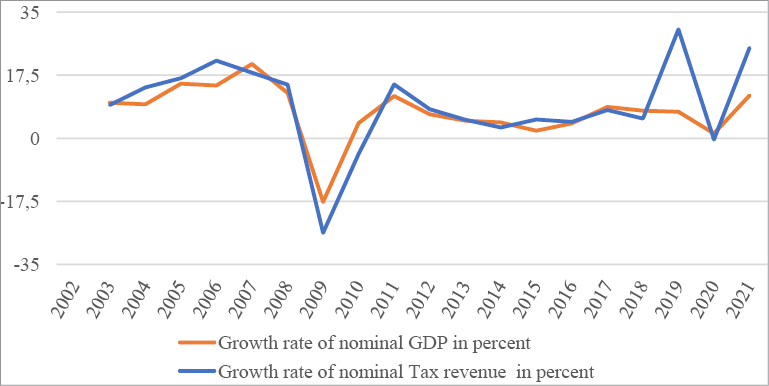
Figure 1 shows the growth rates of nominal gross domestic product (GDP) and total tax revenues in Lithuania from 2002 to 2021. In the periods 2003–2007, 2011–2013, 2015–2016, 2018–2022, the growth rate of tax revenues in Lithuania exceeds the growth rate of GDP.

Figure 1. Growth rates of nominal GDP and tax revenue in Lithuania (in percent)

Source: authors’ calculation, Ministry of Finance of Republic of Lithuania, State Data Agency.

The main tasks of this article are:

• to analyze the tax structure in Lithuania and its interrelation with GDP;

• to create an econometric autoregressive distributed lag model (ARDL) model to analyze the impact of GDP on tax revenues in the short run;

• to extend the created ARDL model with an ECM model, which allows us to analyze long-run effects.

Research of the tax structure in Lithuania and their interrelation with GDP is important for the design and development of tax policy, firstly, because it helps to assess the efficiency of the tax system and to identify its weaknesses. Secondly, because it helps to identify the risk factors in the formation of the government budget, and thirdly, because it allows policy makers to improve the quality of tax revenue forecasts. The objects of this study are the total tax revenues and the tax revenues from different types of taxes, i.e. income tax, corporate tax, value-added tax, excise duties, international trade and transaction taxes in Lithuania. In this paper we used quarterly data of tax revenues and GDP levels in Lithuania from 2002 to 2022 years. An autoregressive distributed lag model (ARDL) was used to analyze the impact of GDP on tax revenues in the short-run, but the ARDL model could not provide a long-run relationship between variables. The long-run effects will be calculated through ARDL model coefficients and using of the long-run multiplier (Blackburne & Frank, 2007).

The paper is developed as follows: the next Section 2 provides a literature review, Sections 3 and 4 provide a description of data and the methodology, the next section analyzes results obtained and the last section provides conclusions and recommendations.

2. Literature Review

The forecast of tax revenues of the state budget in the short and long term is a very important part of a country’s fiscal policy. An inaccurate tax revenue forecast can increase the state budget deficit, and then the government could be even forced to adjust the state budget to not undermine the public’s trust in the implemented fiscal policy. As stated by Cimadomo (2016) and Beetsma et al. (2009) tax revenue forecasting is a complex task, and as such, GDP and tax revenue forecasts are often subject to revisions, creating challenges for the government. To achieve the planned state budget, governments have to change fiscal policy measures and this very rapid correction of the state budget may create a situation where governments will be forced to choose budget correction measures that perhaps are not always most effective. State budget tax revenue forecasts can be applied to total tax revenue or individual revenue sources. Forecasting methods aim to specify and identify the essential relationships between the determinants of taxable capacity and the amounts of revenue actually collected (Göttert & Lehmann, 2021; Ademmer & Boysen-Hogrefe, 2022; Batchelor, 2007).

Tax revenue forecasting must relate to all three variables: tax base, tax rate, and GDP. Generally, a close relationship between taxes and their bases can be expected in the revenue forecast. The size of the corporate tax should depend on the amount of taxable income and the tax rate, and the taxable income should depend on GDP or its components.

Table 1. Contributions to tax revenue analysis

Source: compiled by the authors

Tax revenues of the state budget may change not only due to changes in the tax rate and tax base but also due to conjunctural fluctuations in the gross domestic product. The magnitude and significance of the impact of GDP on tax revenue will vary depending on which part of the business cycle the economy is in, for example, whether in recession or expansion. The economic system has spontaneous stabilizers that mitigate cyclical fluctuations. Self-sustaining stabilizers are self-sustaining fiscal policy measures that increase aggregate demand when the economy is in recession and stem the growth of aggregate demand when the economy is growing. During a recession, the number of people employed, their wages, the profits of enterprises and the turnover of goods are reduced. This reduces the tax base. During the recession, the unemployment rate is usually rising, therefore, unemployment insurance benefits and social benefits for families with insufficient income are increasing. During an economic upturn, the tax base and the average tax rate on personal income increases and social benefits decrease. This dampens the growth of aggregate demand and may cause an overheating of the economy. The advantage of automatic stabilizers over targeted fiscal policies is that they work on their own without prior decisions by the government. However, according to McKay & Reis (2016) self-stabilizing agents cannot eliminate undesirable changes in the equilibrium product. Rather, they only mitigate the amplitude of economic fluctuations. Symansky & Baunsgaard (2009) emphasize that among various taxes, those on income respond the most to the economic cycle, reflecting the progressive rate structure for personal income taxes and the close link to profitability for corporate income taxes. Among Organisation for Economic Co-operation and Development countries (OECD), income taxes can automatically stabilize between 20 and 50 per cent of income shocks (IMF, 2020).

A study of the response to changes in output found that short-run elasticity is higher than the long-run elasticity during economic booms and lower during downturns (Sancak et al., 2010). Other works studying the impact of business cycles on the size of budget revenues and expenditures prove the cyclicality of monetary and tax policy in Latin American countries (Gavin & Perotti, 1997) and developed countries (Kumar & Balassone, 2005). In particular, a 1 per cent increase in the GDP gap leads to a deterioration of budget revenues by 0.2 to 0.5 percentage points of GDP. A study conducted by Kalash et al. (2022) in European Union countries from 2006 to 2018 showed that a 1% increase in GDP increases total tax revenue by 6.91%. Government spending, total investment, and population have positive effects on total tax revenue, and a 1% increase in these factors increases total tax revenue by 2.38%, 0.001%, and 0.57% in these countries. In contrast, inflation, unemployment and gross national savings have a negative impact on all tax revenues, and their growth is 1 per cent reduces the level of total tax revenue by 3.72%, 0.001% and 1.48%.

But there is no consensus on the direction of this relationship. Some studies suggest that tax revenues affect economic growth negatively. Ahmad et al. (2018) researched the empirical relationship between indirect taxes and economic growth in Pakistan. Indirect taxes had a negative and significant effect on economic growth in the long run while its coefficients in the short run were insignificant. Due to a one per cent increase in indirect taxes, economic growth would decrease by 1.68 per cent. Al-tarawneh et al. (2020) determined that there is a negative short- and long-run relationship between taxes and economic growth in Jordan. Other studies emphasize that tax revenues are important for economic growth. Egbunike et al. (2018) find a positive impact of tax revenue on the gross domestic product of Nigeria and Ghana.

Some studies present different effects of taxes on GDP. Gashi et al. (2018) showed that most taxes have a positive effect on GDP growth, but also noted that not all taxes have the same effect on the economic growth of Kosovo. Tax on profits, tax on the individual business, value-added tax, taxation of monthly statements, collection of resources and payment of taxes on interest, dividends, property rights, rentals, lottery and gambling winnings and corporation tax are significant and have a positive impact on Kosovo’s GDP, unlike tax personal and withholding tax which are not significant and have a negative impact on economic growth. Muduli & Manık (2020) examine the impact of tax structure on economic growth in fourteen states of India during 1980–1981 to 2016–2017. The study shows that different taxes have different growth effects. Direct taxes have a negative significant effect on economic growth, but indirect taxes positively influence economic growth because of their nondistortionary effects on the economic system and the productive use of physical and human capital. Mohamed (2022) revealed that all the independent variables had a positive relationship with GDP, but the indirect tax had a negative in Somalia. The study by Ur Rehman et al. (2020) conducted in Asian countries presented that indirect taxes have a positive and significant effect on economic growth in Asia. The tax on goods and services has a positive and significant effect on economic growth in Bangladesh, Iran, Nepal, Turkey, Indonesia, Malaysia, Thailand and Bhutan, while it has a negative and significant effect on economic growth in Pakistan, Sri Lanka, the Philippines and Japan

In recent decades, there has been a noticeable decrease in corporate tax rates in many countries of the world. Due to the significant spread of processes of globalization, the question arises about the impact of integration between countries on corporate taxes. In this context, what is interesting is the so-called tax leadership of the United States, which implies that any corporate tax rates in other countries that exceed similar rates in the United States cannot exist in the long term. This means that in the context of globalization, most countries, due to significant competition for producers, adapt to the corporate tax rates in effect in the United States (Kumar & Quinn, 2012). Since the beginning of the 1980s, in the United States, the corporate tax rate was 47%, while in the late 2010s it was 33%. During the same time period, taxes in South Asia decreased from 55% to 32%, and in all other states from 37–48% to 22–30%. Thus, all countries are trying to lure manufacturers by creating the most favorable conditions for capital (Sokolovska et al. (2020)). We should not forget that similar processes take place in direct competition between neighboring countries.

3. Data

We used quarterly data of tax revenues and GDP levels in Lithuania from 2002 to 2022 (see appendix). We consider the following variables:

• TOTAL_TAX_REVENUE – total tax revenues in Lithuania, th. euros;

• CORPORATE_TAX – corporate tax in Lithuania, th. euros;

• EXCISE_DUTIES – corporate tax in Lithuania, th. euros;

• INCOME_TAX – income tax in Lithuania, th. euros;

• VAT – value-added tax in Lithuania, th. euros;

• GDP_AT_CURRENT_PRICES – GDP at current prices in Lithuania, mln. euros;

The trend of changes in tax revenues of the state budget during the time period of 2002–2021 reflects the cyclicality of the Lithuanian economy (see Fig. 2).

The rate of change of tax revenues at the turning points has a larger impact on changes than the fluctuations of the country’s GDP, but the frequency of fluctuation of tax revenues coincides with the change of the country’s GDP. The year 2019 can be singled out. There have been changes in the tax system in Lithuania, the tax rates and/or tax bases of some taxes have changed, and in 2020 the decrease in tax revenues was influenced by the COVID-19 pandemic. The percentage decrease of tax revenues of the Lithuania budget was a sign of the 2008–2009 crisis (-26.2%), when as a result both the state debt and the budget deficit increased in Lithuania (Fig.3).

Figure 2. Dynamic of total tax revenue and GDP at current prices, percent change

Source: authors’ calculation, Ministry of Finance of Republic of Lithuania, State Data Agency.

Figure 3. Dynamic of different tax revenues and GDP at current prices, percent change

Source: authors’ calculation, Ministry of Finance of Republic of Lithuania State Data Agency.

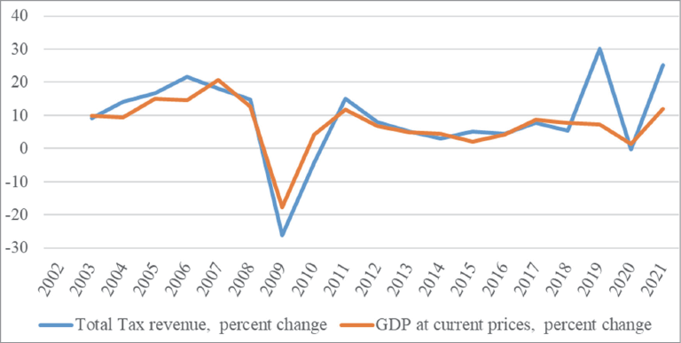
According to Eurostat in 2009 in Lithuania, the ratio of public sector debt to GDP was 29.9 percent (-15.6 percent in 2008). The increase in debt (56.35%) was mainly caused by the increased deficit of the government sector due to the decrease in budget revenues. The size of Lithuania’s state debt, like other economic indicators, was influenced not only by the economic downturn in Lithuania, but also by the economic downturns of other countries with economic ties to Lithuania.

During the time period of 2002–2021, the majority of tax revenue to the state budget was collected from indirect taxes, i.e. VAT, excise duties and International Trade and Transaction taxes (Fig. 4).

Figure 4. Structure of total tax revenues in 2002–2021

Source: authors’ calculation, Ministry of Finance of Republic of Lithuania, State Data Agency

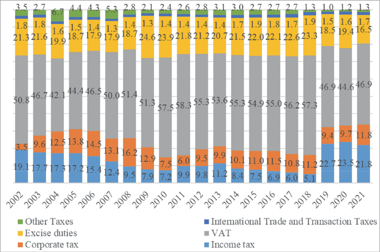
On average, it is about 73.5 percent of total taxes collected. Collected VAT taxes are one of the main sources of budget revenues. The share of this tax in the income structure of the state budget ranges from 42.1 percent (2004) to 58.3 percent (2011), the average is 51.2 percent. Also, a considerable part of the state budget income is made up of excise taxes. The share of tax revenues from excise duties in the structure of state budget revenues ranges from 17.9 (2007) to 24.6 percent (2009) (20.7 percent in average). The share of personal income tax (PIT) and corporate income tax (CIT) in the structure of the state budget income collection is similar: the share of PIT in the structure of state budget income ranges from 5.1 percent (2018) to 23.5 percent (2020), the average is 12 percent, while in CIT from 3.5 percent (2002) to 14.5 percent, the average is 10.7 percent. During 2006 the average is also 10.7 percent. It can be stated that in the structure of tax revenues of the state budget, tax revenues collected from indirect taxes fluctuate the most, i.e. from VAT.

4. Methodology and model estimation.

To begin with, consider the model in the form that was proposed in [1]:

[1]

It is a form of the ARDL model that examines the relationship between tax revenues and a country’s GDP. Later, this model was transformed by the authors into the form of ECM:

Such a view made it possible to conclude on the basis and coefficients, in particular, the value of the coefficient β_i is a parameter of long-run buoyancy of the tax, λ_i is the speed of adjustment, θ_i,0 measures the instantaneous effect of a change GDP on tax revenue, reflecting the short-term buoyancy of the tax. The authors conducted research based on the given model for 34 countries, which did not include Lithuania.

We will study only one country – Lithuania – so instead of the above described regression, we will consider the ARDL model for different types of tax revenues. For its construction, it is necessary to guarantee that all variables are stationary. To do so, we will conduct the Dickey–Fuller stationarity test. As we can see from Table 2, all the studied variables are stationary in first differences, but not stationary in levels. Accordingly, we will select an ARDL model in which all variables will be used in the first differences.

Table 2. Checking variables for stationarity

Source: authors’ calculation

Thus, our final model was

The next stage is the model specification, choosing the best number of lags for each variable. Appropriate parameters were selected based on Akaike’s information criterion. An interesting fact was that all models have the same lag dependence of the tax variable, namely 3 lags were observed. At the same time, the dependence on the influence of economic growth varied significantly. Table 3 shows the estimates of the models.

Table 3. Estimation of the models

*Not significant at 95% of confidence, but significant at 90% of confidence.

Source: authors’ calculation

The current ARDL model cannot provide a long-run relationship between factors. But the actual impact of independent lags can be calculated through model coefficients. Blackburne & Frank (2007) indicated that an approximation of the long-run multiplier can be written in the form

This allows us to calculate the long-run effect of GDP changes to changes in different forms of taxes.

Table 4. Long-run effects

Source: authors’ calculation

The next step of the research is to study the elasticity coefficients, which allows us to analyze the degree of influence of the corresponding lags on the dependent variables. These coefficients show the response as a percentage change in the dependent variable to a 1% change in the according lag from its mean value. The corresponding calculations are given in Table 5.

Table 5. Elasticity coefficients for lags of tax revenues and GDP

Source: authors’ calculation

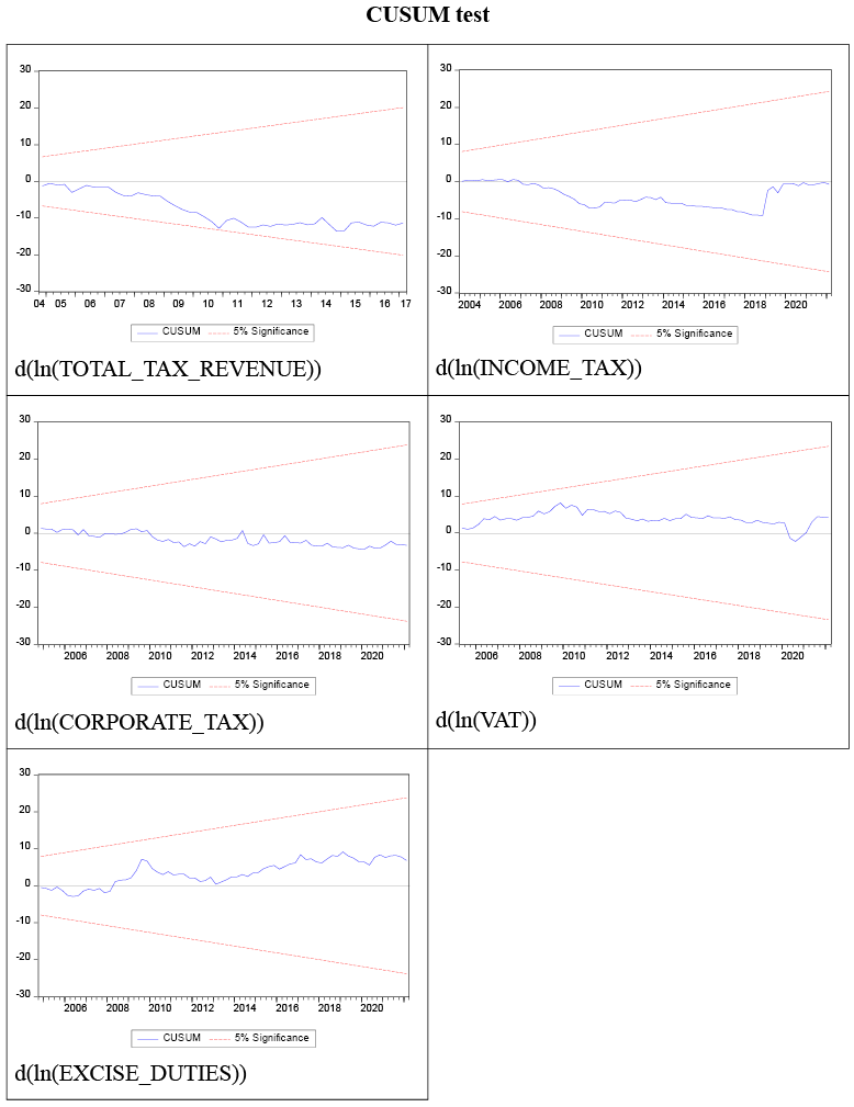
Next, we conduct an analysis using the CUSUM test. This test uses the so-called recursive residuals, which are obtained using the recursive least squares method. The study of the recursive residuals allows us to come to conclusion on the stability of the model parameters, since the mathematical expectation of the stability of the model is zero, and the standard deviation is the standard error of the model. Fig. 5 shows the results of testing, which prove the stability of all proposed models.

Figure 5. CUSUM test

Source: calculated by authors

5. Results

The results of the analysis indicated that in the short-term period, all considered variables have approximately the same behavior. In particular, all considered variables of tax revenues depend on their lags up to and including the third period, which confirms the high inertia of tax revenues.

However, their impact varies significantly. In particular, for total revenues, the influence coefficients vary from -0.54 to -0.88, which indicates a significant level of seasonality. At the same time, the impact of revenues on corporate profits varies from -0.62 to -0.73, which suggests approximately the same level throughout the year. The impact of the lag on excise taxes is significantly decreasing. The strongest impact is observed in the previous period (-0.84), and in the third only only -0.39. The impact of the lag on income from citizens’ incomes, as expected, showed multidirectional dynamics. For the first and third lags, these values were -0.11 and -0.26, respectively, and for the second +0.25. This means that citizens react significantly to changes in their incomes and try to respond flexibly by adjusting their behavior. Absorbed VAT gradually decreases over time from -0.75 to -0.55.

It should be noted that all coefficients were negative, the increase in tax payments in previous periods leads to a decrease in tax revenues in the current period.

The impact of GDP growth turned out to be, as expected, positive. In particular, a quarterly increase in GDP by 10 million euros leads to an increase in total expenditures by 9.32 thousand euros in the current period, 11.97 thousand euros after one period, 6.85 thousand euros after 2 periods and by 8.80 thousand euros after 3 periods. The cumulative effect reaches 36.95 thousand euros or about 0.09% of GDP growth.

The analysis of elasticity coefficients shows that for total tax revenues, in most cases, the impact of GDP growth is sufficiently proportional to the growth of taxes. At least on average, the values of elasticity coefficients for GDP are very close to 1. This means that certain fluctuations are possible during different periods, but these fluctuations balance each other out. Elasticity coefficients for lags show a downward trend in absolute value, remaining negative. This means that the impact of changes in tax revenues is gradually losing its impact. However, all these coefficients are less than 1 in absolute value, which means that their influence has a residual inert character.

At the same time, for most taxes, the elasticity coefficients for GDP are less than 1, that is, the increase in GDP growth by 1% leads to an increase in tax growth by less than 1%. The only exception to this rule is VAT, which makes it possible to balance the insufficient impact of all taxes.

The long-term effect of changing factors is thus interesting and relevant for the analysis. For total tax revenues, this effect is equal to 1.187, which means that the Lithuanian tax system has significant opportunities to increase tax collection, at least by 18.7% of tax growth. The most ripe candidate for an increase in tax collections is the corporate income tax. With proper administration, it is possible to achieve a growth rate of 2.16 times the current level of growth. Revenues from excise taxes will be the least prone to growth.

Conclusions

The degree of dependence between the level of economic development and the payment of taxes is a fundamental feature of the economic development of the state and its competitiveness. On the one hand, a high level of taxation contributes to income being hidden in the shadow economy. This characterizes low-income countries. As an economy grows, the level of taxes paid should also increase, which allows for a reduction in tax rates, thereby stimulating tax revenues in the long term. As a result of globalization, this process takes place in most countries of the world, which means that countries become actual competitors among themselves in tax rates. Less developed countries try to reduce tax rates to attract large enterprises, which will in the future pay large tax amounts of revenue into the national budget. It is therefore not surprising that EU and the United States reached agreements on the lower limit of certain types of taxes, in particular, income tax, which makes endless competition impossible.

At the same time, the tax payment process is characterized by a rather large state of inertia. Businesses and individuals are not ready to quickly change their behavior in tax evasion, which makes quick reforms in this area impossible.

The paper examines the question of how exactly this inertia manifests itself in Lithuania. Based on the 2002–2002 data, an ARDL model was constructed, which made it possible to determine the short-term effect on tax revenues of various types of taxes when GDP changes.

We have shown that for all types of taxes except value-added tax, this effect is smaller than GDP growth in the current period. The effect of GDP growth on total revenues have diverse dynamics over 3 periods. Considering that all other taxes have the effect of increasing tax revenues less than the growth of the tax base, it can be concluded that the level of general tax collection is administratively regulated by the government, allowing for relaxation and strengthening of tax collection, especially for enterprises.

Examining the long-term impact of changes in GDP showed that an increase in GDP has a positive effect on almost all types of taxes. At the same time, it should be noted that the long-term effect for general taxes is almost 19% higher than the growth of the tax base, that is, the Lithuanian economy as a whole tends towards an expansion of the shadow economy. This effect is most pronounced for the corporate tax, where the effect is higher than the growth of the tax base by 115%. It is obvious that we are referring to the elimination of the shadow economy of the corporate sector both through administrative means and through psychological factors when after a certain level of income, it becomes less profitable to avoid paying taxes.

For personal income tax, the effect is not so high – only about 7%, which indicates that the elimination of the shadow economy will not be very rapid for this tax. Excise tax stands separately, for which GDP growth in the long term does not contribute very effectively to filling the budget. This means that the consumption of excise goods will not grow in proportion to GDP, and therefore this tax can only have a corrective function.

Thus, from a policy point of view of flow management, the Lithuanian government should continue the strategy of reducing the shadow economy, especially in the corporate sector.

References

Ademmer, M., & Boysen-Hogrefe, J. (2022). The Impact of Forecast Errors on Fiscal Planning and Debt Accumulation. Jahrbucher Fur Nationalokonomie Und Statistik, 242(2), 171–190. https://doi.org/10.1515/jbnst-2020-0054

Ahmad, S., Sial, M. H., & Ahmad, N. (2018). Indirect Taxes and Economic Growth: An Empirical Analysis of Pakistan. Pakistan Journal of Applied Economics, 28(1), 65–81. https://doi.org/10.21859/eulawrev-08062

Al-tarawneh, A., Khataybeh, M., & Alkhawaldeh, S. (2020). Impact of Taxation on Economic Growth in an Emerging Country. International Journal of Business and Economics Research, 9(2), 73. https://doi.org/10.11648/j.ijber.20200902.13

Andrejovska, A., & Pulikova, V. (2018). Tax revenues in the context of economic determinants. Montenegrin Journal of Economics, 14(1), 133-141. https://doi.org/10.14254/1800-5845/2018.14-1.10

Batchelor, R. (2007). Bias in macroeconomic forecasts. International Journal of Forecasting, 23(2), 189-203. https://doi.org/10.1016/j.ijforecast.2007.01.004

Bayar, Y., & Ozturk, O. F. (2018). Impact of foreign direct investment inflows on tax revenues in OECD countries: A panel cointegration and causality analysis. Theoretical & Applied Economics, 25(1). http://www.ectap.ro/articol.php?id=1318&rid=130

Benedek, M. D., Gemayel, M. E. R., Senhadji, M. A. S., & Tieman, A. F. (2021). A post-pandemic assessment of the sustainable development goals. International Monetary Fund.

Beetsma, R., Giuliodori, M., & Wierts, P. (2009). Planning to cheat: EU fiscal policy in real time. Economic policy, 24(60), 753-804. https://doi.org/10.1111/j.1468-0327.2009.00230.x

Blackburne, E. F., & Frank, M. W. (2007). Estimation of Nonstationary Heterogeneous Panels. The Stata Journal: Promoting Communications on Statistics and Stata, 7(2), 197–208. https://doi.org/10.1177/1536867X0700700204

Castañeda Rodríguez, V. M. (2018). Tax determinants revisited. An unbalanced data panel analysis. Journal of Applied Economics, 21(1), 1-24. https://doi.org/10.1080/15140326.2018.1526867

Castro, G. Á., & Camarillo, D. B. R. (2014). Determinants of tax revenue in OECD countries over the period 2001–2011. Contaduría y administración, 59(3), 35-59. https://doi.org/10.1016/S0186-1042(14)71265-3

Cimadomo, J. (2016). Real‐time data and fiscal policy analysis: A survey of the literature. Journal of economic Surveys, 30(2), 302-326. https://doi.org/10.1111/joes.12099

Egbunike, F. C., Emudainohwo, O. B., & Gunardi, A. (2018). Tax Revenue and Economic Growth: A Study of Nigeria and Ghana. Signifikan: Jurnal Ilmu Ekonomi, 7(2), 213–220. https://doi.org/10.15408/sjie.v7i2.7341

Gavin, M., & Perotti, R. (1997). Fiscal policy in latin america. NBER macroeconomics annual, 12, 11-61. https://doi.org/10.1086/654320

Gashi, B., Asllani, G., & Boqolli, L. (2019). The effect of tax structure in economic growth. International Journal of Economics and Business Administration, 7(1), 56–67. https://doi.org/10.35808/ijeba/209

Göttert, M., & Lehmann, R. (2021). Tax Revenue Forecast Errors: Wrong Predictions of the Tax Base or the Elasticity? SSRN Electronic Journal, June. https://doi.org/10.2139/ssrn.3872387

Imam, P. A., & Jacobs, D. (2014). Effect of corruption on tax revenues in the Middle East. Review of Middle East Economics and Finance, 10(1), 1-24. https://doi.org/10.1515/rmeef-2014-0001

International Monetary Fund. (2020, April 15). Fiscal Monitor „Policies to Support People During the COVID-19 Pandemic“.

Kalaš, B., Đurović-Todorović, J., & Đorđević, M. (2020). Panel estimating effects of macroeconomic determinants on tax revenue level in European Union. Industrija, 48(3), 41–57. https://doi.org/10.5937/industrija48-27820

Kalaš, B., Mirović, V., & Andrašić, J. (2020). Cointegration analysis of indirect taxes and economic growth in the Republic of Serbia. Anali Ekonomskog Fakulteta u Subotici, 35(44), 3–10. https://doi.org/10.5937/aneksub2044003k

Kumar, M., & Balassone, F. (2005). Cyclicality of Fiscal Policy and Cyclically Adjusted Fiscal Balances. SM/05/393. Washington, International Monetary Fund.

Kumar, M. S., & Quinn, D. P. (2012). Globalization and Corporate Taxation. IMF Working Papers, 12(252), 1. https://doi.org/10.5089/9781557754752.001

McKay, A., & Reis, R. (2016). The role of automatic stabilizers in the US business cycle. Econometrica, 84(1), 141-194. https://doi.org/10.3982/ECTA11574

Mohamed, A. K. (2022). The Impact of Tax Revenue on Economic Growth in Somalia. Journal of Economics and Sustainable Development, 13(2), 62–70. https://doi.org/10.7176/JESD/13-2-07

Ministry of Finance of Republic of Lithuania. https://finmin.lrv.lt/lt/aktualus-valstybes-finansu-duomenys/valstybes-biudzeto-ir-savivaldybiu-biudzetu-vykdymo-duomenys

Minh Ha, N., Tan Minh, P., & Binh, Q. M. Q. (2022). The determinants of tax revenue: A study of Southeast Asia. Cogent Economics & Finance, 10(1). https://doi.org/10.1080/23322039.2022.2026660

Muduli, D. K., & Manık, N. (2020). Tax structure and economic growth in general category states in India: A panel auto regressive distributed lag approach. Theoretical and Applied Economics, 27(2), 225-240. https://store.ectap.ro/articole/1464.pdf

Raouf, E. (2022). The impact of financial inclusion on tax revenue in EMEA countries: A threshold regression approach. Borsa Istanbul Review, 22(6), 1158-1164. https://doi.org/10.1016/j.bir.2022.08.003

Saptono, P. B., & Mahmud, G. (2021). Macroeconomic Determinants of Tax Revenue and Tax Effort in Southeast Asian Countries. Journal of Developing Economies, 6(2), 253. https://doi.org/10.20473/jde.v6i2.29439

Sancak, C., Xing, J., & Velloso, R. (2010). Tax Revenue Response to the Business Cycle. IMF Working Papers, 10(71), https://doi.org/10.5089/9781451982145.001

Sokolovska, A., Zatonatska T., Stavytskyy, A., Lyulyov, O., Giedraitis, V. (2020) The Impact of Globalization and International Tax Competition on Tax Policies. Research in World Economy. Vol. 11, No. 4 (Special Issue). Doi: https://doi.org/10.5430/rwe.v11n4p1.

Symansky, S. A., & Baunsgaard, T. (2009). Automatic fiscal stabilizers. IMF Staff Position Notes, 9, 23. International Monetary Fund.

State Data Agency. https://osp.stat.gov.lt/nacionalines-saskaitos

Tsaurai, K. (2021). Determinants of tax revenue in upper middle-income group of countries. The Journal of Accounting and Management, 11(2). https://dj.univ-danubius.ro/index.php/JAM/article/view/864

Tsaurai, K. (2021). Tax Revenue and Economic Growth in Emerging Markets: Is Financial Development Relevant? The Journal of Accounting and Management, 11(1), 134–144. https://dj.univ-danubius.ro/index.php/JAM/article/view/498

Ur Rehman, Z., Khan, M. A., & Muhammad Tariq, M. (2020). Indirec Taxation and Economic Growth Relationship: Empirical Evicence from Asian Countries. Pakistan Journal of Humanities and Social Sciences Research, 3(01), 131–144. https://doi.org/10.37605/pjhssr.3.1.11

Appendix

Tax revenues and GDP in Lithuania

Source: Ministry of Finance of Republic of Lithuania, State Data Agency