Ekonomika ISSN 1392-1258 eISSN 2424-6166

2024, vol. 103(1), pp. 6–24 DOI: https://doi.org/10.15388/Ekon.2024.103.1.1

In the Context of Okun Law, the Relationship Between Real Output and Unemployment Rate in Oecd: a Panel Error Correction and Panel Ardl Approaches

Utku Altunöz
Sinop University, Turkey
Email: utkual@hotmail.com
ORCID: https://orcid.org/0000-0002-0232-3108

Abstract. In this paper, the correlation between unemployment rate and real output for OECD countries was analyzed through the application of Okun’s Law and unemployment hysteresis 2007-2022. For this purpose, panel error correction, panel cointegration, ARDL Bounds Test and Granger causality techniques were preferred. In addition, unemployment hysteresis was examined with different panel unit root technique in OECD countries. The findings show that there is a long-term link among the variables, while supporting unemployment hysteresis in most OECD countries. Long-term findings show that Okun’s law is applicable. Causality analysis indicates that there is a one-way and negative relationship towards the unemployment rate. The estimation for the long-run coefficient shows that the increase in growth leads to a decrease in the unemployment rate. Short-term findings also support long-term outcomes.
Keywords: Okun, unemployment, output.

_________

Received: 25/02/2023. Revised: 20/03/2023. Accepted: 18/04/2023
Copyright © 2024 Utku Altunöz. Published by Vilnius University Press
This is an Open Access article distributed under the terms of the Creative Commons Attribution License, which permits unrestricted use, distribution, and reproduction in any medium, provided the original author and source are credited.

Introduction

Unemployment is seen as a multifaceted fundamental problem with both economic and social dimensions. The unemployment problem poses a greater threat especially for developing countries that are disadvantaged in terms of economic growth and development. The high level of unemployment constitutes a dimension of production below the potential production level. This situation causes the labor, which is a valuable production factor for production, to remain idle in economies where there is already a lack of resources for developing countries. This situation forms the basis for seeing the unemployment problem as a priority problem for developing economies. Policy makers are trying to take measures to resolve unemployment, which is one of the common problems of both developed and developing economies. Reducing rising unemployment rates back to reasonable levels becomes both a very difficult and time-consuming issue due to the rigidity in the labor markets. Following the 2008 Global Financial Crisis; European countries have also had to implement policies regarding the regulation of the labor market to find a measure for increasing unemployment rates (Heimberger, 2019: 1).

The sensitivity of unemployment rates to economic activity depends on some factors (such as labor market conditions, regulations ...). Labor market dynamics, as emphasized in classical economic theory is not a market structure that is balanced under full employment conditions depending on wage and price flexibility. The existence of structural unemployed, mainly caused by wage rigidity, and frictional unemployed caused by temporary factors, hinders the clearing of the labor market.

Especially in the period from the 1960s to the mid-1970s, the growth rate in OECD countries such as Germany, France and England reached 3.5% and the unemployment rates fell to around 3-4% (Üzar and Akyazı,2018:466). In the same period, the USA showed a lower growth performance compared to these countries and the unemployment rate was realized at the level of 6-7%. With the beginning of the 1980s, while the growth rate in Germany and France fell below 2%, the unemployment rate increased to 9%. By the 1990s, the economic growth in the USA increased to approximately 3.5% and the decrease in unemployment rates to 5% has created an important consensus on the validity of Okun Law (Khemraj et al., 2006: 4).

With the implementation of labor market flexibility practices since the 2000s, it is seen that the share of temporary employment in employment has increased in most of the OECD countries. While standard employment relations are permanent and permanent; Temporary employment type covers jobs with a certain deadline. Individuals in some temporary employment forms work under a subcontractor rather than obeying the orders and instructions of a single employer and cannot benefit from wide legal regulations such as minimum wage, unemployment insurance, protection against dismissal, unlike standard employment forms (Cuyper et al., 2008, p. 27). Therefore, short-term employment forms have an employment structure that leads to a reduction in the time spent at work. However, since 2006, it is seen that the time spent at work (job stability) has increased in some countries. This is due to the higher labor force sharing of the elderly population because of the abolition of early retirement programs and the raising of the corporate retirement age in many OECD countries in recent years. The fact that older individuals have spent a longer time at work (seniority) leads to a longer period spent at work by the workforce. Ignoring this factor, length of stay decreases by more than 17% in Sweden, Luxembourg, and Lithuania. (ILO, 2019: 96).

The global financial crisis deeply affected the advanced and emerging economies. The macroeconomic instability and high unemployment rates experienced during this period brought the discussion on the determinants of unemployment back to the agenda. The contractionary impacts of the global crisis and the continuing uncertainty in the world economy decreased investment, trade, and thus global aggregate demand. In accordance with the data of the ILO, the unemployment rate in the world economy in 2016 is 5.7% and the number of unemployed is approximately 200 million (ILO, 2017: 5). According to the OECD, global gross domestic product will shrink by 4.5% in 2022 and increase by 5% next year. The Paris-based organization said that by the end of 2022, production in many countries will be below the levels at the end of 2019 and well below what was predicted before the pandemic.

Various investigations have found that the link between unemployment rates and economic growth is not linear. For this reason, this relationship also analyzed with the Markov regime change model to make the study stronger.

Studies on Okun’s Law in the literature generally focus on a single country. The aim of this study is to reveal the effects of the Covid epidemic and the Russia-Ukraine war by adding current data to the analysis of the validity of Okun’s law for the Turkish economy. In this respect, it is thought that the study will make an original contribution to the previous literature. In addition, panel error correction and panel cointegration techniques were preferred in the analysis of the relationship between the variables. In addition, unemployment hysteresis was examined with different panel unit root technique for unemployment hysteresis in OECD countries. The rest of the paper is designed as follows:

Theorical Background

The main factor that determines the long-term connection between the unemployment rate and the GDP growth rate is the growth rate of the potential output level. The growth rate of potential output shows an improvement depending on the potential productivity and the growth rate of the labor supply when the economy operates in full employment conditions. When the unemployment rate is high, current gross domestic product potential level below the level and therefore an output gap occurs. The growth rate of output equates to the growth rate of the labor supply under conditions where there is no productivity growth and every new participation in the labor force translates into employment. However, when the growth rate of gdp stays below the growth rate of the labor force, the employment rate of the labor force decreases. In contrast, the unemployment rate declines in the long run when the GDP growth exceeds the growth rate of the labor force and the productivity growth rate (potential output) (Levine 2013). Okun (1962) reveal that real GDP growth is 1% above the 2.25% trend value and reduces the unemployment rate by 0.5%. In Okun’s study, the values cover the American economy, and the annual population growth rate is around 1%. (Altunöz,2019:200). Okun (1962) used three models to confirm his claims. These patterns are known as first differences, test exploits, and proper propensity and elasticity. In the first difference method, quarterly changes in unemployment rate (Y) and GNP (X) are correlated as percentages. Projected from 55 observations from 1947:2Q to 1960:4Q. The result is the following equation (1):

Y = 0,30 – 0,30X (1)

In equation (1), 1% increase in GDP causes a 0.3-point decrease in the unemployment level. The relevant regression equation is determined with an arrow. The unemployment equation is as in equation (2) below.

U = a + b (deficit) (2)

The findings achieved in the models performed by Okun submitted to the joint economic committee in 1961 as equation (3).

U = 3.72 + 0.36 (Deficit) (3)

Equation (3) expresses that unemployment is 3.72% in an economy where there is no current account deficit. Okun (1962), in based on the US economy, analytically demonstrated the inverse connection between potential output and unemployment rate, depending on the change in working time, labor force participation and productivity. (Holmes and Silverstone, 2006:293).

The last part of the Okun is called appropriate disposition and flexibility. While the first part focuses on the change in unemployment and GNP, the following section is based on the level values s, assuming that the growth trend in the second method is the constant unemployment rate. (Altunöz,2019:202).

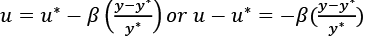
Okun states that if the real output differs from the potential, the connection on how the unemployment rate will be affected (i.e. to what extent the real unemployment will differ from the full employment unemployment will be as equation (4) below.

(4)

In equation (4), u is the real unemployment , u* is the natural unemployment, y is the real product, and y* is the potential real product. Apart from this original formulation, the Okun relationship can be considered as a correlation between the real and potential output growth and the change in the unemployment as equation (5) follows:

∆u = –β(y – y*) (5)

Undoubtedly, the coefficient β may be different for various economies or at several times in the similar economy. There are also some obstacles in calculating u* and y* values. However, Okun’s law, which is called a law and not an empirical regularity; It provides a practical method for converting the growth rate of output to the reduction in the unemployment rate. Even though this rule is only estimate and does not run very accurately from year to year, it still provides a meaningful conversion from growth to unemployment (Dornbusch and Fischer, 1998:19).

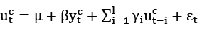
Moosa (1997) used the cyclical output gap and the cyclical unemployment while examining the association between unemployment rates and GDP within the framework of Okun’s law. The model created by Moosa (1997) can be represented as equation (6) follows:

(6)

In equation 6, is the cyclical unemployment rates and is the cyclical output gap. The divergence of real GDP from the trend value was calculated by the Hodrick Prescott method. The lagged value of the cyclical unemployment rate was added to the model to avoid the autocorrelation problem(Barışık at al.,2010: 92). The β coefficient shown is called the Okun coefficient and the long-run relationship between the cyclical output gap and the cyclical unemployment rate is calculated as θ = β/(1 – γ). However, the literature that has developed in recent years indicates the presence of a non-linear relationship mentioned variables.. For example, for Cuaresma (2003), Holmes and Silverstone (2006), Barışık at al. (2010), Viren (2001) found that the relationship between unemployment rates and economic growth is not linear. For this reason, the correlation among variables was investigated with the Markov regime change model.

Literature

Christopoulos (2004) investigated the correlation between the variables in Greece. According to the results of the analysis, it was concluded that Okun’s Law is not valid in 7 of 13 regions. Akram at al. (2014) examined whether the Okun Law was applicable in Pakistan. In this study, data between 1972 and 2012 were used. As a result, it has been determined that there is a causal relationship between economic growth and unemployment. In her study, Tatoğlu (2017) investigated the validity of the OKUN Law for European countries between 2008 and 2016, with the (4D) panel data model. The validity of Okun’s Law was tested both based on countries and for the whole panel, and the Okun coefficient was calculated. As a result, it was found that Okun’s Law is valid in European Countries and Okun’s coefficient is around -0.09. In addition, Okun’s Law applies in 13 of the 23 countries studied. The increase in youth unemployment rate has been a major problem for many European countries in recent years. Dunsc(2017) analyzes age- and gender-specific unemployment rates in Central and Eastern European countries using Okun’s law, and shows that young people in Central and Eastern European countries are predominantly more sensitive to business cycle fluctuations, regardless of gender. Moosa (1999) tried to estimate the Okun coefficient with the Dynamic ARDL (autoregressive distributed lag) method in the period 1947: Q1-1992: Q2 in the United States and found the Okun coefficient -0.16 for the short term and -0.38 for the long term. In other words, he determined that increasing economic growth had a decreasing effect on the unemployment rate. The author also showed that there is no structural break in the relationship between unemployment and GDP. Sögner and Stiassny (2000) used the Kalman filtering method and Bayesian analysis, which considers structural breaks for fifteen OECD countries and determined that the effect of the change in economic growth on the unemployment rate differs for countries other than Italy. Altunöz (2015) worked with the data of the period 2000: Q1- 2014:Q1 to analyze the validity of Okun’s Law for Turkey in the context of real growth and unemployment, and as a result of the analysis; He concluded that there is no cointegration relationship between real growth and unemployment series, that is, there is no long-term relationship between these series. As a result of Granger causality analysis, it was seen that there was no causality relationship between these series. As a result of variance decomposition, while growth influences the formation of unemployment, it has been found that unemployment does not have a significant effect on growth. Villaverde and Maza (2009), in their study covering sub-regions of Spain, investigated the relationship between unemployment rate and growth using quadratic, Hodrick-Prescott and Boxter-King filtering methods and found that there was a difference between unemployment and growth for many regions. They concluded that there is an inverse relationship. However, they found that the Okun coefficient varies according to the regions. Grant (2018) analyzed Okun’s law in the context of potential output and natural unemployment rate and found a significant time variation in the Okun coefficient in the USA. Altunöz (2019) examined the validity of the Okun Law for the Euro Region in the annual panel data set covering the period 2000-2012 and concluded that the Okun Law is acceptable. Nevertheless, the coefficient of cointegration is smaller than the Okun coefficient determined for the USA and other studies conducted for advanced countries. Erdoğan at al. (2019) analyzed the period of 1923-2015 with piecewise regression analysis. The findings showed that Okun’s Law was valid between the years 2000-2015, which is the second sub-period. Chuttoo (2020) analyzed the relationship between unemployment and economic growth in Mauritius with the ARDL cointegration test and concluded that there is a negative cointegration between economic growth and unemployment both in the long run and in the short run, but it is not statistically significant. From the Okun coefficient obtained, it is concluded that a 4 percent change in the gross domestic product (GDP) growth rate in Mauritius changes the unemployment rate by 1 percent in the opposite direction. In their study, Bod and Považanová (2020) examine the different asymmetries in Okun’s law for 21 OECD countries over the period 1989–2019. For most countries, Okun’s law manifests itself more strongly in years when output is much lower than in years when output increases. In almost all countries, Okun’s law is found to be stronger with falling unemployment, and weaker or balanced by rising unemployment. Using new sectoral data, Goto and Burigi (2021) estimated the Okun’s law at the sector level for the USA, England, Switzerland, and Japan, and concluded that the Okun coefficients follow similar patterns to the total Okun coefficients across countries. Özer (2022) In his study, which analyzes the validity of Okun’s law for the Turkish economy with the fractional frequency Fourier ARDL bounds test method, with quarterly time series for the period 2007-2022, there is a one-way negative relationship from growth to unemployment in both the long and short run. In addition, Okun’s law is strongly supported. Elhorst and Emili (2022) analyzed Okun’s law for the Dutch economy with two dynamic spatial panel data models, in which output growth and the change in unemployment rate are interrelated, and concluded that the relationship of Okun’s law from output growth to unemployment dominates in their study.

Methodology

In this study, we examine the validity of Okun’s Law in the context of the relationship between unemployment rate and real output in the OECD, taking into account unemployment hysteresis, with quarterly time series data covering the period 2007: Q2- 2022:Q2.The change in real gross domestic product compared to the previous period was used to represent economic growth (g_t), and the harmonized unemployment rate (un_t) was used to represent the unemployment rate. Seasonally adjusted quarterly series were obtained from the FRED (Federal Reserve Bank of St. Louis) database.

For the empirical analysis of the Okun law by Okun, 2 types of models are proposed. One of them is the first difference model and the other is the gap model. In the first difference model, the correlation between (g_t) and (un_t) is examined within the context of the following function as equation (7) (Villaverde and Maza, 2007: 8)

g_t – g_t–1 = α + β(un_t –un_t–1) + μ_t (7)

The β, which is estimated to be fewer than zero in Equation (7), is the Okun coefficient and measures the impact of differences in the (un_t) on real (g_t). μ_t is White noise (random walk) term with zero mean and constant variance. Equation (7) is acceptable and true under either the hypothesis that they are cointegrated to avoid spurious regressions, or that all the series in parentheses are stationary. The second definition for the arrow’s law is the gap model. The gap model obtained by using equation (7) can be followed in equation (8).

(8)

In equation (8), g^*_t is the logarithm of the long-run level of output (potential output) and the natural (un_t). Other parameters are compatible with equation (7). On the left side of equation 8, the first term, left t, represents the difference between observed and potential (un_t) (unemployment gap), while (g – g^*_t ) represents the (g_t) gap equal to the observed and potential (g_t) difference. (Real GDP).

According to Doğru (2013), the unemployment hysteresis hypothesis has a permanent effect on the (un_t) level due to the labor market rigidities of cyclical fluctuations.

Unit root examinations offer a procedural context for analytically determining the hysteresis hypothesis. If the (un_t) series has a unit root, we assume that it has a permanent effect on it. The hysteresis hypothesis states that (un_t) contain a unit root, in other words, they are not stationary. For this purpose, panel unit roots will be preferred in the study.

If time series are subject to econometric analysis, it is expected that each variable does not have a unit root, in other words, they are stationary. Otherwise, encountering the spurious regression problem will prevent the analysis from giving accurate results. For this reason, unit root tests have attracted attention in recent years for those working with panel data.

Cross-section Dependency Tests

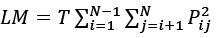
One of the tests that should be done before unit root tests in panel analysis is horizontal dependency tests. Cross-section independence is based on the idea that all countries subject to analysis have the same degree of impact from the shock that will occur in any of the units that make up the panel, and that the macroeconomic shock that may occur in any country does not affect the other countries in the panel. It is an undeniable reality that the macroeconomic developments in the countries in the global world, the exchange rate shocks affect the other countries that trade with that country, and even the geography where the country is located. Therefore, the estimation results obtained in panel analyzes where the cross-sectional dependence is not considered may be inconsistent and biased. In this context, the existence of cross-section dependence between the series should be tested (Menyah et al. 2014:389). The first of the tests developed to investigate the existence of cross-sectional dependence is the Lagrange Multiplier (LM) test developed by Breusch and Pagan (1980) and seen in equation (9).

(9)

In equation (9), P represents the binary correlation of the residuals as a sample estimate.

In the Lagrangian Multiplier (LM) test, two different hypotheses are established, the null hypothesis and the alternative hypothesis H₀=no relationship between horizontal sections and alternative hypothesis H₁: There is a relationship between cross-sections.

In the absence hypothesis, when T → ∞ is assumed that n constant degrees have the asymptotic distribution of degrees, and the time dimension of the test will be preferred if the horizontal cross-sectional size of T is greater than N. The test in question was developed by Pesaran (2004) and named as CD_LM in the literature and is expressed as in equation (10).

(10)

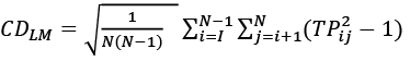
In equation 10, it is claimed that there is no cross-section dependence in the case of T→∞ and N→∞. However, in cases where N>T, the CD_LM test shows deterioration in the level, so again Paseran (2004) developed the CD test, which is valid in cases where >T, and equation (11) can be followed.

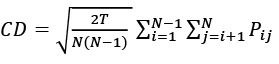(11)

Another cross-section dependency test is Pesaran and Yamagata. (2008) is the LM_adj test and equation (12) can also be followed.

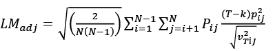(12)

While the regressor numbers are expressed with k in Equation (5), is the avarage of

For these tests:

(H₀) claims the absence of cross-section dependency, while (H₁) claims its existence.In cases where the H₀ is rejected the analysis continues with first-generation panel unit root tests, while in case of cross-section, second-generation panel unit root tests are used (Baltagi, 2008: 284).

Table 1. Cross Section Tests

Test	Statistic	Probability
LM (Breusch ve Pagan,1980)	20,11	0,00
CDLM (Pesaran, 2004)	1,76	0,01
CD (Peseran, 2004)	-0.67	0,02
LMadj (Peseran vd. 2008)	1,91	0,00

In Table 1 to test the homogeneity of the slope coefficients, H₀ stating no cross-sectional dependence in the countries subject to the sampling is accepted at 99% significance level. According to the result obtained, it can be said that the effect that will occur in any of the countries that are the subject of the analysis will not affect the other countries. Therefore, in the next part of the analysis, first generation panel unit root tests should be applied. In this context, Levin, Lin and Chu (2002), and Im, Paseran, Shin (2003), panel unit root tests will be preferred.

Panel data analysis results can be obtained by combining individual unit root tests in Im, Pesaran and Shin (2003) panel unit root test. In this unit root test developed for heterogeneous panel data analysis, heterogeneity is allowed between cross-sections (countries, etc.). A separate ADF is determined for each cross-section and the hypotheses in the panel unit root test of Im, Pesaran and Shin (2003) are tested with equation (13).

(13)

The hypotheses of the unit root test are as in equation (14) and equation (15).

H₀ = α₁ = 0 (14)

H₁ = α₁ < 0 (15)

It is in the form. Levin, Lin, Chu (2002) unit root test, the basic ADF formulation in equation (16) is used.

(16)

Levin, Lin, Chu (2002) unit root test, the null and alternative hypothesis are as in equation (17) and equation (18).

H₀: α₁ = 0 (17)

H₁: α₁ < 0 (18)

Levin, Lin, Chu (2002) unit root test, the null hypothesis in equation (17) is tested and there is a common unit root.

Table 2. Im, Paseran, Shin Unit Root Results (dependent variable: un_t)

Variables	Model	t Statistic	Result
unt	constant	-5,145*	I(I)
	constant and trend	-4,018	I(I)
gt	constant	-6,718**	I(I)
	Constand and trend	-2,891**	I(I)

Note: * and ** respectively; It expresses significance at the 1% and 10% level.

For the Im, Paseran, Shin Unit Root Test presented in Table 2, both constant and constant and trend models were used. Lag lengths were determined by the Schwartz Information Criteria. Considering the results obtained, both variables have unit root and they are I(I)

Levin, Lin, Chu results can be seen in Table 3. The lag lengths were determined by the Schwartz Information Criteria.

Table 3. Levin, Lin, Chu Unit Root Results (dependent variable: un_t)

Variables	Model	t Statistic	Result
unt	constant	-7,101**	I(I)
	constant and trend	-5,578**	I(I)
	constant and non-trend	-5,208**	I(I)
gt	constant	-4,239*	I(I)
	constant and trend	-3,308*	I(I)
	constant and non-trend	-2,255*	I(I)

According to the results each series I(1)in all the constant, constant and trended and non-trend models in the series. In other saying, H₀ is not rejected. The fact that both different tests give the same result means that the variables subject to the analysis are not stationary in the series but stationary in I(I). And Augmented Dickey Fuller (ADF) and Phillips–Perron (PP) unit root tests are employed for each country individually as can be seen in Table 4 and Table 5. The lag orders are automatically chosen by Akaike information criterion (AIC).

According to the results of the individual unit root tests applied to each country separately (Table 4 and Table 5), the (Un) series is stationary at the first difference at a significance level of at least 10 % in all countries except Iceland. In other words, the real output series are stationary for all countries except Iceland and Ireland.

The econometric estimation method we used in the empirical analysis of this study are co-integration analyzes and vector error correction (VEC) techniques. Several recent studies take a more contemporary approach to establishing a VEC model by identifying the relationship between the I (1) series.

Table 4. ADF Individual Test

Countries	Augmented Dickey Fuller Unit Root
	unt		gt
	level	1st difference	level	1st difference
Austria	0,172	0,013	1,222	0,010
Belgium	0,301	0,012	1,001	0,008
Canada	0,192	0,001	0,171	0,044
Denmark	0,200	0,001	1,190	0,011
France	0,291	0,021	0,291	0,021
Germany	0,167	0,016	0,167	0,016
Greece	0,811	0,024	0,811	0,024
Iceland	0,081	0,017	0,081	0,017
Ireland	0,209	0,001	0,006	0,000
Italy	0,110	0,009	4,211	0,024
Luxembourg	0,191	0,008	2,240	0,022
Netherlands	0,221	0,009	2,101	0,010
Norway	0,267	0,014	3,310	0,002
Portugal	0,111	0,009	0,291	0,021
Spain	0,191	0,014	0,167	0,016
Sweden	0,188	0,088	0,188	0,088
Switzerland	0,361	0,021	1,200	0,001
Turkey	0,412	0,016	1291	0,021
United Kingdom	0,211	0,024	0,167	0,016
United States	0,240	0,022	0,240	0,022

Table 5. PP Individual Test

Countries	Phillips–Perron test Unit Root
	unt		gt
	level	1st difference	level	1st difference
Austria	0,166	0,010	1,091	0,000
Belgium	0,222	0,002	2,023	0,002
Canada	0,180	0,006	0,166	0,031
Denmark	0,188	0,006	1,017	0,001
France	0,179	0,011	0,291	0,021
Germany	0,180	0,011	0,167	0,016
Greece	0,101	0,002	0,811	0,024
Iceland	0,011	0,002	0,081	0,017
Ireland	0,180	0,006	0,006	0,000
Italy	0,188	0,006	4,211	0,024
Luxembourg	0,121	0,001	2,240	0,022
Netherlands	0,110	0,002	2,101	0,010
Norway	0,200	0,032	3,310	0,002
Portugal	0,100	0,005	4,314	0,000
Spain	0,166	0,010	0,180	0,013
Sweden	0,129	0,060	0,178	0,006
Switzerland	0,410	0,012	1,333	0,022
Turkey	0,789	0,024	0,188	0,006
United Kingdom	0,333	0,020	0,121	0,001
United States	0,129	0,022	0,110	0,002

In a VEC model, the first difference of the variables included in the model is represented as a function of their lagged values, the lagged values of other explanatory variables, and the cointegration equation. A simple VEC model with bivariate
g_t and un_t and lag length of 1 can be written as follows (Doğru,20213:97).

(19)

(20)

In equations (19) and (20), where t represents years, ∆g_t is the first difference of the logarithm of real output and ∆ un_t is the first difference of the logarithm of the unemployment rate; ε'_1t–1 = g_t–1 – γ₁ – θ₁un_t is the one-year lagged “disequilibrium residuals” from the related cointegration equations. Also, α, γ and θ are the parameters to be predicted, k is the lag length and ε determine the errors term (ET).

Pedroni’s (1999) cointegration test will be preferred to test the validity of the long-run relationship among the variables. In this context, cointegration statistics, excluding for the group p-test in table 5, support evidence for the steady-state balance between real output and unemployment rate in the long run. The cointegration relationship implies that there is a causal interaction between the variables under analysis. In this context, a panel vector error correction (VEC) model can be created and estimated using equations (14) and (16) because, econometrically, we know that a VAR model that includes the lagged values of the dependent and independent variables and the error correction term (ECT) (equal to the VEC model) is estimated when the variables given in the (15) and (16) model are cointegrated.

Table 6. Panel Co-integration Results

Within dimension test	intercept	intercept and trend
Panel v statistics	0,21	-0,57
Panel rho (p)-statistic	1,80	-0,02*
Panel PP statistic	-5,11**	-9,11*
Panel ADF statistic	-2,33	-5,66*
Between dimension test
Group rho(p)-statistic	1,51*	1,99*
Group PP-statistic	2,76**	-8,21*
Group ADF- statistic	1,25*	-5,21

**and * respectively indicates the statistical significance at 1 and 5 levels.

Table 6 provides evidence for the steady-state balance among variables in the long run in all the cointegration statistics. The cointegration correlation indicates a causal interaction between unemployment and output. In the next step, the estimation results of the long- and short-term panel estimation results based on VECM estimation can be viewed in Table 7.

Table 7. Panel Short and Long Term VECM estimation result

	Short Term	Long Term
Variables	∆un	∆g
∆un	-	0,64(0,58)
∆g	0,10(0,081)	-
Error Correction Term
	ECT un	ECT g
	-0,55*	-0,48*
Panel Cointegration equation: git = –0,579unit + μit

The VEC model estimation is presented in Table 7. The results show that the ECT has taken a negative and statistically significant value and there is a long-term relationship among the variables subject to the analysis. In this context, the cointegration coefficient to be reached by estimating the cointegration equation will express the coefficient of the long-term Okun. This long-run relationship is as follows in Table 8. The Okun coefficient was also estimated by the Least Square (FMOLS) and Dynamic Ordinary Least Square (DOLS) methods established by Pedroni (2000 and 2001) to make the analysis in the study strong and reliable. Long-term cointegration coefficients are as Table 8.

Table 8. Panel Cointegration Test Results

	un	g
Panel Dynamic Ordinary Least Square (DOLS)	-0,061*	-0,011*
Panel Fully Modified Ordinary Least Square (FMOLS)	-0,066*	-0,030*

Note: * denotes statistical significance at the 1% level.

According to the results, (un) is negatively correlated with (g) in the long run in both DOLS and FMOLS. In addition, according to the Panel DOLS estimation result, a 1 % reduce in (g) increases the (un) by 0.061 percent, while a 1 % increase in (g) decreases the (un) by 0.011 %. FMOLS estimation results show that a 1 % decrease in real (g) increases the (un) by 0.030 %, and a 1 % increase in (un) is associated with a 0.066 % decrease in real (g).

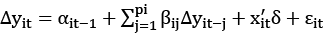
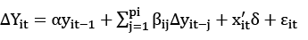
To strengthen the empirical analysis and increase its reliability, the panel ARDL test will also be applied to the variables. The general form of the panel ARDL(p,q) model can be seen in equation (21).

(21)

In Equation (21), the vector of the dependent variable is expressed with Y_i,t while the vector of the independent variable is expressed with X_i,t In the analysis of cointegration relations, the problem of deviation from long-term balances is encountered. For this reason, with the help of error correction model (ECM), short-term relationships and how long it takes for short-term deviations to reach equilibrium can be analyzed. The ECM to be applied for this purpose can be followed in equation (12).

(22)

In Equation (22), the short-run coefficients are expressed with ω_ij and δ_ij. Where β represents the long-run coefficients, ∅_i represents the ECT. The ECT is expected to be between 0 and 1 and negative.

The ECT is expected to be between 0 and 1 and negative. Paseran et al. (1999) developed two estimators for the ARDL model, namely the Pooled Mean Group estimator (PMG) and the Mean Group Estimator (MG). MG does not place any limits on the ARDL definition variable. It also derives its long-term definitions from the long-term definition mean from ARDL estimates. The shortcoming of said estimator is that it does not allow certain parameters to be the same among the units that make up the panel. This deficiency is eliminated by the PMG estimator. Hausman type tests are preferred to decide whether the obtained prediction coefficients are heterogeneous or homogeneous.

If the obtained results show homogeneity, the PMG estimator is more efficient than the MG (Mean Group) estimator, which allows heterogeneity. In other words, PMG estimator should be preferred in case of homogeneity of long-term coefficient estimations, and MG estimator in the opposite case. While determining the optimal number of delays in the analysis, the Akaike information criterion was used and it was understood that the appropriate model was ARDL (4,3). The long-term ARDL equation is as in equation (23).

(23)

Long-term ARDL estimation results in the study can be seen in Table 9.

Table 9. Panel ARDL Long Run Estimation Results

Long Run	PMG	MG	Hausman
un	-1,312*(0,00)	-1,112*(0,00)	chi square (7)=5.17
c	34,111**	31,110**(0,00)	Probability = 0,58

Note: (*) and (**) denote significance at the 1% and 5% levels, respectively.

According to the results in Table 7, obtained from the Hausman test, it was understood that the coefficients were homogeneous. According to the results obtained, it was decided to use the PMG estimator. The long-term coefficients were found to be statistically significant. Accordingly, a 1 % in (g) causes a 1,312 % decrease in (un) in the long run. Diagnostic test results related to the long-term model are presented in Table 10.

When the results in Table 10 are examined, it is seen that there is no problem of varying variance (ARCH LM Test) and autocorrelation (Breusch-Godfrey LM Test) in the model. In addition, it is observed that the ET has a normal distribution (Jarque-Bera Normality Test) and there is no model building error (Ramsey Reset Test). After the long-term results, short-term results based on the ET have been estimated, and the obtained short-term results can be viewed in Table 11.

Table 10. Diagnostic Tests for Long Run

Diagnostic Tests	Coefficient
R2	0,900
Adjusted R2	0,901
F stat	365,112(0,000)
Breusch – Godfrey Test	1,689(0,4212)
ARCH LM Test	0,130(0,400)
Jarque – Bera Normality Test	1,311(0,316)
Ramsey Reset Test	2,011 (0,212)

Table 11. Panel ARDL Short-Term Estimation Results

Short Run	PMG	MG
un	-0,097*(0,00)	-0,082*(0,00)
ECT	-0,25**(0,00)	-0,27**(0,03)
C	-0,68*(0,57)	-4,67(7,18)

Note: (*) and (**) denote significance at the 1% and 5% levels, respectively.

When the findings are analyzed in Table 11, it is seen that the short-term coefficient is statistically significant. Accordingly, a 1% rise in g_t causes a 0.089 % fall in (un) in the short run. Therefore, it is possible to state that (g) has a negative effect on (un) both in the short and long and short run. However, this effect is large in the long run and very small in the short run. The ECT coefficient was found to be negative and statistically significant. This shows that the dynamic equilibrium condition is met and the deviations from the short-term equilibrium disappear spontaneously in the long-term. Accordingly, 0,25 % of a short-term imbalance is compensated. In other words, the imbalances occurring in the short term come to equilibrium after 4 periods (approximately 1 years).

Table 12. Diagnostic Tests of the Short-Term Model

Diagnostic Tests	Coefficient
R2	0,948
Adjusted R2	0,900
F stat	362,288(0,000)
Breusch – Godfrey Test	1,600(0,3200)
ARCH LM Test	0,102 (0,654)
Jarque – Bera Normality Test	1,214(0,506)
Ramsey Reset Test	2,011 (0,212)

According to the diagnostic findings in Table 12, it is realized that there are no autocorrelation, functional form and varying variance problems in the ARDL model. In addition, according to the results, it is revealed that the errors show a normal distribution.

The CUSUM and CUSUMSQ tests performed to test the structural breaks and stability of the parameters of the econometric analysis, in other words, to determine the stability of the model, can be seen in Figure 1.

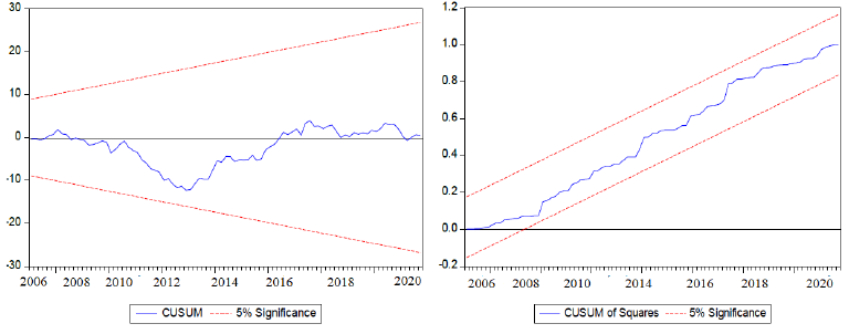
Figure 1. CUSUM ve CUSUMQ Testi

According to Figure 1, since the solid line remains within the limits indicated by the dashed lines at the 5% significance level, it is understood that the parameters are stable and there is no structural change. In econometric studies, causality analyzes are preferred to understand whether two variables are in a causal relationship. The Granger causality test is established on the regression model in Equations (24) and (25).

(24)

(25)

In equations (24) and (25), while u expresses ET, lag lengths are expressed with m.

Table 13. Granger Causality Test Results

Aspect of Causality			F Stat.	Probability/ Result
g	→	un	6,11*	0,000 / Accept
un	→	g	0,10	0,412 /Reject

In Table 13, it is seen that economic growth is Granger causal of unemployment, that is, (g) affects (un), but (un) is not Granger causal of (g).

Conclusion

We investigate the connection between unemployment rate and real output in OECD over the implementation of Okun’s Law and unemployment hysteresis by quarterly series over the period of 2007- 2022. Panel error correction and panel cointegration techniques were preferred for the analysis of the relationship among the variables. In addition, unemployment hysteresis was investigated by different panel unit root technique for unemployment hysteresis in OECD countries. According to the results obtained, there is a proof supporting unemployment hysteresis in most of the OECD countries.

The long-term coefficients were found to be statistically significant. Accordingly, a 1 % in economic growth causes a 1,312 % reduce in unemployment in the long run. Accordingly, a 1% rise in economic growth causes a 0.089 % fall in unemployment in the short run. Therefore, it is possible to state that economic growth has a negative effect on unemployment both in the short and long and short run. However, this effect is large in the long run and very small in the short run. The ECT coefficient was found to be negative and statistically significant. This shows that the dynamic equilibrium condition is met and the deviations from the short-term equilibrium disappear spontaneously in the long-term. Accordingly, 0,25 % of a short-term imbalance is compensated. In other words, the imbalances occurring in the short term come to equilibrium after 4 periods (approximately 1 years). it is seen that economic growth is Granger causal of unemployment, that is, economic growth affects unemployment , but unemployment is not Granger causal of economic growth. Findings show a long-run relationship among the variables. The long-run findings show that Okun’s law is applicable. The long-term findings are lower than Okun’s coefficient for the USA.To raise the power and reliability of the study, ARDL bounds test was applied to the variables, and it was determined that there is a one-way and negative relationship from economic growth to unemployment rate in the long run. The estimation for the long-term coefficient shows that the increase in growth leads to a decrease in the unemployment rate. Short-term findings also support long-term results.The error correction coefficient, which was found to be statistically significant, reveals that the imbalances occurring in the short term come to equilibrium spontaneously after 4 periods (approximately 1 year). The empirical analysis results obtained support the studies of Dunsc(2017), Altunöz (2015), Altunöz (2019), Bod and Považanová (2020), Goto and Burigi (2021), Özer (2022), Elhorst and Emili (2022). The results of the analysis show that, despite the employment growth phenomenon that emphasizes the weakening of the growth-employment relationship, Okun’s Law is still an important theoretical framework and an important guide for policy makers. While countries can prevent unemployment by increasing economic growth and creating new employment opportunities, they can also ensure that increased employment increases economic growth. In this context, increasing the quality of economic growth, increasing the expenditures that will increase human capital such as education and health, strengthening the real production economy that emphasizes the industry, supporting areas with high value-added production especially for developing countries, and structural reforms will never be very important for growth and employment performance. should not be forgotten. The findings obtained from the causality test also supported the results obtained from the cointegration analysis and confirmed the existence of a unidirectional connection between the variables from economic growth to unemployment rate. Therefore, in the contraction period when the conjuncture slows down, positive effects on employment should be created by applying economic policies that increase growth. This article is a contribution to a better understanding of the OECD labor market at an aggregate level. However, it is thought that the study can be improved with models in which nonlinear situations are used in future studies.

References

Maza, A. &Villaverde, J. (2007). Okun’s law in the Spanish regions. Economics Bulletin, 18(5), 1–11.

Akram, Misbah, et al. (2014). An Empirical Estimation of Okun’S Law in Context of Pakistan. Journal of Finance and Economics, 2(5), 173-177. https://doi.org/10.12691/jfe-2-5-7

Altunöz, U. (2015). Reel Büyüme ve İşsizlik Bağlamında Türkiye İçin Okun Yasası Analizi. Kamuİş, 14(1), 29–44.

Altunöz, U. (2019). The Relationship between Real Output (Real GDP) and Unemployment Rate: An Analysis of Okun’s Law for Eurozone. Sosyoekonomi, 27(40), 197–210. https://doi.org/10.17233/sosyoekonomi.2019.02.12

Barışık, S., Çevik, E.İ., Çevik, K.,N. (2010). Türkiye’de Okun Yasası, Asimetri İlişkisi ve İstihdam Yaratmayan Büyüme : Markov-Switching Yaklaşımı. Maliye Dergisi, 159, 88–102.

Bod’a, M. and Považanová, M. (2021). Output-unemployment asymmetry in Okun coefficientsforOECD countries. Economic Analysis and Policy Volume 69, 307–323, https://doi.org/10.1016/j.eap.2020.12.004

Breusch, T. and Pagan, A. (1980). The Lagrange Multiplier Test and Its Applications to Model Specification in Econometrics. Review of Economic Studies, 47(1), 239–253. https://doi.org/10.2307/2297111

Chrıstopoulos, D. (2004). The relationship between output and unemployment: evidence from Greek regions. Papers in Regional Science, 83(3), 611–620. https://doi.org/10.1007/s10110-004-0198-y

Chuttoo, U.D. (2020). Effect of Economic Growth on Unemployment and Validity of Okun’s Law in Mauritius. Global Journal of Emerging Market Economies, 12(2), 231–250. https://doi.org/10.1177/0974910119886934

Cuaresma, J. C. (2003). Okun’s Law Revisited. Oxford Bulletin of Economics and Statistics, 65(4), 439–451. https://doi.org/10.1111/1468-0084.t01-1-00056

Cuyper, N.L. & Jong, J. & Witte, H.D & Isaksson, K. & Rigotti, T. & Schalk, R. (2008). Literature Review of Theory and Research on The Psychological Impact of Temporary Employment: Towards A Conceptual Model. International Journal Of Management Reviews, 10(1), 25–51. https://doi.org/10.1111/j.1468-2370.2007.00221.x

Doğru,B. (2013). The link between unemployment rate and real output in Eurozone: A panel error correction approach. Procedia - Social and Behavioral Sciences, 99, 94–103. https://doi.org/10.1016/j.sbspro.2013.10.475

Dunsch,S. (2017). Age- and Gender-Specific Unemployment and Okun’s Law in CEE Countries. Eastern European Economics, 55(4), 377–393, https://doi.org/10.1080/00128775.2017.1338962

Erdoğan, S., Yıldırım, D. Ç., Kırcı Çevik, N. & Tosuner Ünal, Ö. (2019). Okun yasasının geçerliliği: Türkiye’den ampirik bulgular. Maliye Dergisi, 177, 70–86.

Elhorst, P.J. and Emili, S. (2022). A spatial econometric multivariate model of Okun’s law. Regional Science and Urban Economics, 93. https://doi.org/10.1016/j.regsciurbeco.2021.103756

Grant, A.L. (2018). The Great Recession and Okun’s law. Economic Modelling Volume 69. https://doi.org/10.1016/j.econmod.2017.10.002 291-300.

Goto, E. and Bürgi, C. (2021). Sectoral Okun’s law and cross-country cyclical differences. Economic Modelling, 94, 91–103, https://doi.org/10.1016/j.econmod.2020.08.016

Heimberger, P. (2019). The Impact of Labour Market Institutions and Capital Accumulation on Unemployment: Evidence for the OECD, 1985-2013. The Vienna Institute for International Economic Studies, Working Paper: 164.

Holmes, M.J. and Silverstone, B. (2006). Okun’s Law, Asymmetries and Jobless Recoveries in the United States: A Markov-Switching Approach. Economics Letters, 92, 293–299. https://doi.org/10.1016/j.econlet.2006.03.006

ILO (2017). World Employment and Social Outlook: Trends 2017. Geneva, Switzerland: International Labour Office-ILO.

ILO (2019). World Employment and Social Outlook: Trends 2019. Geneva, Switzerland: International Labour Office-ILO.

Im, K.S., Pesaran, M.H. and Shin, Y. (2003). Testing for unit roots in heterogeneous panels. Journal of Econometrics, 115(1), 53–74. https://doi.org/10.1016/S0304-4076(03)00092-7

Khemraj, T., Madrıck, J. and Semmler, W. (2006). Okun’s Law and Jobless Growth. Schwartz Center For Policy Analysis, The New School Policy Note, 3, 1-10.

Levin, A., Lin, C. and Chu, C. (2002). Unit root tests in panel data: Asymptotic and finite-sample properties. Journal of Econometrics, 108(1), 1–24. https://doi.org/10.1016/S0304-4076(01)00098-7

Levine, L. (2013). Economic Growth and the Unemployment Rate. Congressional Research Service.

Menyah, K., Nazlıoğlu, S. and Wolde-Rufael, Y. (2014). Financial Development, Trade Openness and Economic Growth in African Countries: New Insights from a Panel Causality Approach. Economic Modelling, 37, 386–394. https://doi.org/10.1016/j.econmod.2013.11.044

Moosa, I.A. (1997). A Cross-Country Comparison of Okun’s Coefficient. Journal of Comparative Economics, 34, 335–356.

Moosa, I.A. (1999). Cyclical Output, Cyclical Unemployment, And Okun’s Coefficient A Structural Time Series Approach. International Review of Economics and Finance, 8, 293–304.

Okun, A.M. (1962). Potential GNP: Its Measurement and Significance. Reprinted as Cowles Foundation Paper.

Özer, M. O. (2022). Ekonomik Büyüme ve İşsizlik Oranı Arasındaki İlişki: Kesirli Frekanslı Fourier ARDL Sınır Testi Yaklaşımı. İstanbul İktisat Dergisi, 72(1), 269–292. https://doi.org/10.26650/ISTJECON2022-1020006

Paseran, M.H; Sin, Yongcheol; Smith, Ron P. (1999). Pooled mean group estimation of dynamic heterogeneous panels. Journal of the American Statistical Association, 94(446), 621–634. https://doi.org/10.1080/01621459.1999.10474156

Paseran, M. Hashem. (2004). General Diagnostic Tests for Cross Section Dependence in Panels. University of Cambridge Working Paper.

Pedroni, P. (1999). Critical Values for Cointegration Tests in Heterogeneous Panels With Multiple Regressors. Oxford Bullettin of Economics and Statistics, Special Issue, 653-670.

Pedroni, P. (2000). Fully-modified OLS for heterogeneous cointegrated panels. Advances in Econometrics, 15, 93–130. https://doi.org/10.1016/S0731-9053(00)15004-2

Pedroni, P. (2001). Purchasing power parity tests in cointegrated panels. Review of Economics and Statistics, 83(4), 727–731. https://doi.org/10.1162/003465301753237803

Pesaran, M.H. (2007). A Simple Panel Unit Root Test İn The Presen-Ce Of Cross Sectiondependence. Journal Of Appliedeconometrics, 22(2), 265–312.

Pesaran, M.H. and Yamagata, T. (2008). Testing Slope Homogeneity in Large Panels. Journal of Econometrics, 142(1), 50–93. https://doi.org/10.1016/j.jeconom.2007.05.010

Sögner, L. and Stiassny, A. (2000). A Cross-Country Study on Okun’s Law. Vienna University, Working Paper Series, No:13.

Tatoğlu, F.Y. (2017). A nalysis of Okun’s Law with Multi-DimensionalPanel Data Models in European Countries. Journal of Management and Labour, 1(1),43–56.

Üzar, U. and Akyazı, H. (2018). Ekonomik Büyüme ve İşsizlik Arasındaki İlişkinin OECD Ülkeleri Düzeyinde Ekonometrik Bir Analizi. Cumhuriyet Üniversitesi İktisadi Ve İdari Bilimler Dergisi, 19(2), 463–479.

Villaverde, J. and Maza, A. (2009). The Robustness of Okun’s Law in Spain, 1980-2004: Regional Evidence. Journal of Policy Modeling, 31, 289–297. https://doi.org/10.1016/j.jpolmod.2008.09.003

Viren, M. (2001). The Okun Curve is Non-linear. Economics Letters, 70, 253–257. https://doi.org/10.1016/S0165-1765(00)00370-0