Organizations and Markets in Emerging Economies ISSN 2029-4581 eISSN 2345-0037
2021, vol. 12, no. 1(23), pp. 51–70 DOI: https://doi.org/10.15388/omee.2021.12.47

Fiscal Policy, Monetary Policy and Price Volatility: Evidence from an Emerging Economy

Le Thanh Tung
Policy and Applied Economics Research Group, Faculty of Economics and Public Management, Ho Chi Minh City Open University, Ho Chi Minh City, Vietnam
tung.lt@ou.edu.vn
https://orcid.org/0000-0001-8487-2217

Abstract. Vietnam is an Asian emerging country, which now is ranked in the group of the fastest-growing economies worldwide. However, this economy has faced galloping inflation in recent years. So the Vietnamese experience is a valuable reference for the policymakers in the developing world in order to successfully control price volatility. Our study applies the Vector autoregressive method, the Johansen cointegration test, and the Granger causality test to examine the impact of fiscal and monetary policy on price volatility in Vietnam with a quarterly data sample collected over the period from 2004 to 2018. The study results confirm the existence of a long-term cointegration relationship between these policies and price volatility in Vietnam. Besides, the variance decomposition and impulse response function also show that the impact of these policies on inflation is clear, however, the fiscal policy more strongly affects inflation than the monetary policy. Finally, the Granger causality test also indicates one-way causality relationships from the government expenditure as well as the exchange rate to price volatility in the study period.

Keywords: price volatility, inflation, fiscal policy, monetary policy, emerging economy, Vietnam

Received: 25/11/2020. Accepted: 22/3/2021
Copyright © 2021 Le Thanh Tung. Published by Vilnius University Press. This is an Open Access article distributed under the terms of the Creative Commons Attribution Licence, which permits unrestricted use, distribution, and reproduction in any medium, provided the original author and source are credited.

1. Introduction

The governments and their economic policies are popular study topics in macro-economics in order to improve the efficiency of public activities. The economic policies are the activities that governments use to control or monitor the economic behaviors in the market. The operating of policy is a really complex process because an economic policy always has many different effects (both expected and unexpected dimensions) covering the economy. So there are many different results regarding the impact of an economic policy found by empirical studies in countries (Owoye & Onafowora, 1994; Favero & Monacelli, 2003; Cioran, 2014; Hossain, 2014; Hassan, 2015; Martínez-López, 2017). Based on the economic literature, fiscal and monetary policy are the most important tools of government to drive the economy to achieve its goals such as a high growth rate or a dynamic business environment. However, many aspects of the impact of fiscal and monetary policy on other macro-economic indicators (for example, inflation) are not identified or calculated (see Mikek, 2008; Bouakez et al., 2014). Additionally, the policymakers are faced with many planning situations in the economic environment in the context of globalization, which can make the domestic market become more increasingly sensitive to the policy signals. There are some forecasting results that imply policymakers in developing countries will continually face pressures caused by outside business cycles in the context of globalization. So empirical studies in a specific country or a group of countries still have important roles which help to have policy implications to reference in both policy making process as well as academic research.

The economic reforms since 1986 (named as the ‘Doi Moi’ economic renovation) have transformed the Vietnamese economy from one of the poorest in the world to a middle-income country. The average economic growth has been approximately 6.4% per year for this period. In 2020, the Gross domestic product (GDP) of Vietnam was approximately calculated at $340 billion. In terms of GDP size, Vietnam was ranked as the 4^th largest economy in Southeast Asia and the 35^th in the world. Besides, based on the statistics of the General Statistic Office of Vietnam (GSO), in 2019, the population of this country was approximately 96.2 million, and the labour force accounted for 51.4% (around 49.4 million), with the unemployment rate only 2.3% of the labour force (GSO, 2020). Because of many achievements in economic development, in 2005, Vietnam was added to a group of eleven emerging countries called ‘The Next Eleven’. This group includes Bangladesh, Egypt, Indonesia, Iran, Mexico, Nigeria, Pakistan, Philippines, Turkey, South Korea, and Vietnam. The economists of the Goldman Sachs Investment Bank have forecasted the Next Eleven would become the largest economic region in the world in the 21^st century (Wilson & Stupnytska, 2007). Vietnam was also listed to another group of six emerging countries in 2009 (named as ‘CIVETS’), which had Colombia, Indonesia, Vietnam, Egypt, Turkey, and South Africa. The CIVETS is expected as a new economic growth motivation of the world economy in the next decades (McGregor, 2011). The Vietnamese economy is really a potential market, where the businesses can have high performing as well as many opportunities caching enormous profit (Hoa et al., 2020; Tung, 2020).

However, after a long period having fast and stable growth, the Vietnamese economy has been faced with some macro problems in recent years. For example, the economic growth rate slowed down, and inflation robustly increased in the same period. Based on the statistics of the General Statistics Office of Vietnam, the average rate of economic growth was 8.05% per year in the period of 2003-2007 and sharply dropped to 5.93% per year in the period of 2008-2012; after that, the average growth rate was recovering at 6.2% per year in 2013-2017. As a negative result, economic growth adopted an unstable trend compared to the previous decade.

During the period of 2008-2012, the number of corporate bankruptcies significantly rose, and the decline of GDP increased the unemployment rate of the economy. The main problem which might harm the Vietnamese economy was inflation. Obviously, the statistics showed that price strongly fluctuated in this period. The inflation (calculated by the consumer price index) ran at the moderate level of 5.1% per year and stayed in a stable trend in the period of 1993-2002; however, in 2007, the Vietnamese inflation was rapidly rising up to the double-digit level which was called ‘the galloping inflation’. In more detail, the average inflation rate in 2007-2011 increased remarkably by 13.6% per year.

In particular, the inflation rate reached a new record of 18.87% in 2008 as well as 18.13% in 2011 (GSO, 2020). On the other hand, since 2008, the economic growth rate was sharply slowed down and fell in an instability period. In order to decrease the general price level, during this period, Vietnam’s government employed some urgent solutions for coping with high inflation. However, the contractionary policies used to reduce the inflation rate might also suffocate the growth of the economy. After adapting some suitable solutions, in the period of 2012-2018, the inflation rate was trending downward and came back again to a moderate level of 3.8% per year. We can see more detail about the annual inflation rate in this period in Figure 1.

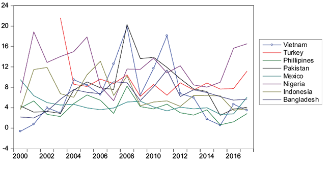
Figure 1. The annual inflation rate in emerging economies in 2000-2017 (Unit: %)
Source: World Bank (2021)

In the period 2003-2018 (especially the years before and after the Global Financial Crisis of 2008), the Vietnamese government applied some expansionary economic policies in order to promote economic growth more rapidly as well as support the modernization progress. In particular, the fiscal policy and monetary policy were the most important and most often used at this period. In the government’s system of Vietnam, the fiscal policy is implemented by the Ministry of Finance, and the monetary policy is operated by the Central Bank. However, the real effective performance of the policies in Vietnam has not been studied enough, at least in the field of practical reference. There are many opposing arguments that can lead to confusion in policy making, thus, the Vietnamese policymakers need to know clearly about the effects as well as roles of these policies in Vietnam with both the positive aspect (e.g., expand production and support growth) and the negative impact (e.g., the price may strongly fluctuate). Besides, the experiences in the battle against inflation in Vietnam are very useful for policymakers in the developing countries in order to have good policies for supporting growth as well as holding macro-economic indicators stable. Furthermore, the review of the literature shows that there is no evidence for the case of Vietnam. Obviously, there is a research gap in the effect of fiscal and monetary policy on price fluctuation in this economy. Therefore, our results will contribute to filling this research gap as well as providing some recommendations for the Vietnamese policymakers to successfully control inflation in the next period. Furthermore, our investigated results are expected to provide some valuable implications for high inflation countries in particular, as well as the developing countries in general.

There are some questions that involve the relationship between the government policies and price fluctuation in the case of Vietnam, the examples are: “What is the effect of fiscal and monetary policy on price fluctuation in Vietnam?” or “Do the fiscal and monetary policy have a role in the price fluctuation in Vietnam?” or “Do fiscal policy and monetary policy cause price fluctuation?”. On the other hand, Vietnam is a highlighted country in the group of the fastest-growing economies, so the investigated result of our paper is a good reference source for policymakers in other countries. The structure of our article includes 5 sections. Section 2 is the overview of the literature and the discussion for some empirical studies. Section 3 represents the econometric methodology and data description. The estimated results and discussion are shown in Section 4. Finally, Section 5 includes conclusions and policy recommendations.

2. Literature review

Following the literature of the economic theories, fiscal and monetary policy are significant tools to express the government’s (or policymakers) opinions in order to control and drive the economic indicators. In particular, the monetary policy is operated by the government’s control in the money supply (Mankiw, 2009, p. 83) and may be related to the adjustment of the nominal exchange rate. For example, the central bank manages the nominal exchange rate based on a managed float regime (as Vietnam); when the central bank increases the nominal exchange rate, after that, the depreciation of the domestic currency may suddenly increase the price of imported goods, causing a rise in the general price level (Mankiw, 2009, p. 358). Meanwhile, the fiscal policy is implemented using two main tools including taxes and government expenditures (Mankiw, 2009, p. 312). Expansionary fiscal policy is implemented on the principles which have a tax reduction and an increase in the government expenditure; on the other hand, an increase in tax and a decrease in the government expenditure is called a contractionary fiscal policy. If the government increases its money supply, that indicates an expansionary monetary policy is implemented, meanwhile, when the money supply is decreased, it means a contractionary monetary policy is performed. Because of the important roles of these public policies they are the usual studying objects in both developed countries and developing countries. However, most of the empirical results are focused on analyzing the impact of these policies on supporting economic growth. In the field of coordination between fiscal and monetary policy, the empirical studies also provide some references for policymakers to be more efficient in controlling the support of the economic growth of the economy. These policies as well as inflation are important macro issues that attract much concern not only from policymakers but also from academic researchers worldwide.

There are some studies that confirm the existence of the relationship between fiscal-monetary policy and inflation, or between these policies and the fluctuation of the general price level in the economy. However, these results are generally inconsistent or even contrary. In the case of the developed economies, Favero and Monacelli (2003) employed the Vector autoregressive (VAR) method for a fiscal policy rule and control for the endogenous regime switches for both rules in the US economy before and after 1987. The result pointed out that in the pre-1987 period, the model based on the two rules explained the behavior of inflation better than the one based just on the monetary policy rule. After 1987, when fiscal policy was estimated to switch to a regime of fiscal discipline, the monetary-fiscal mix could be appropriately described as a regime of monetary dominance. The authors concluded that a monetary policy rule-based model was always a better predictor of inflation behavior than the one comprising both a monetary and a fiscal rule. In another study in the USA, Traum and Yang (2010) applied a new Keynesian model to analyze the fiscal-monetary policy regimes from 1955 to 2007. The estimated result showed that an increase in government spending could induce a positive consumption state in a passive fiscal policy regime. The authors also concluded that an income tax cut could yield a negative labor response if monetary policy aggressively stabilized output.

In the European region, Cioran (2014) examined the existing connections between the inflation rate and some important macroeconomic indicators and also the dynamics of inflation in Romania and the European region. The paper demonstrated the causal relationship between inflation and monetary policy (interest rate) and the causal relationship between unemployment and inflation. Besides, Ćorić, Šimović and Deskar-Škrbić (2015) used the VAR model to analyze the possibilities of monetary and fiscal policy in price stability and economic growth in Croatia in the period 2004-2012. The results indicate that the expansionary monetary and fiscal policies both have positive impacts on economic activities. The fiscal expansion leads to the nominal exchange rate appreciation, while monetary expansion has a depreciation impact on the nominal exchange rate. The articles found that fiscal and monetary authorities could stimulate economic growth without endangering price stability. Fan, Minford and Ou (2016) explored whether the Fiscal Theory of the Price Level (FTPL) could explain the UK inflation in the 1970s. The result showed that fiscal policy had a substantial role in determining inflation. They also found a similar model account for the 1980s; however, the role of fiscal policy was much diminished.

Focusing on the case of the Pacific region, in Australia, Hossain (2014) did an overview of the operation of the monetary policy and pointed out the persistence and volatility of inflation under successive monetary policy regimes in the period of 1950-2010. The result implied that high inflation persistence and volatility suggested that inflationary shock takes a long time to dissipate but does not permanently alter the low average level of inflation in the Australian economy. Lapukeni (2015) focused on the impact of financial inclusion on monetary policy effectiveness in Malawi. The author applied the VAR model and the Granger causality test. Contrary to the economic theories, the study revealed that the money supply had an inverse relationship with inflation.

Besides developed countries, there are some studies that investigated developing countries (especially in Asia and Africa), however, the results were not united in the implications for the policymakers. Owoye and Onafowora (1994) also used the VAR method to examine the relative importance of monetary and fiscal policy in ten African countries with annual data from 1960 to 1990. The result pointed out that the monetary policy was more important than fiscal policy in five countries. In the Turkish case, Tekin-Koru and Özmen (2003) examined the long-term relationships between budget deficits, inflation, and monetary growth. The result showed the joint endogeneity between money (or monetary policy) and inflation in this economy. Blanchard (2004) argued that inflation targeting could have perverse effects in the case of the Brazilian economy. The result implied that an increase in the real interest in response to higher inflation led to a real depreciation, after that the real depreciation led in turn to a further increase in inflation. The paper concluded that the fiscal policy (not monetary policy) was the right instrument to decrease inflation. In the case of Latvia, Tkacevs (2006) studied the indirect impact of fiscal policy on the general price level. The regression result was obtained by the VAR model and the impulse response functions. The result found evidence of Latvian general government budget balance. The result implied that the deterioration of the budget balance could lead to an upward price adjustment in order to assure fiscal solvency.

Besides, Vargas (2012) tried to present empirical evidence regarding the relation of money growth (understood as the monetary policy) and its effect on inflation in Bolivia in the period of 1998-2010. The evidence confirmed that the level of current inflation had a strong relationship with the level of money quantity in the economy. Furthermore, the results also indicated that the expansionary monetary policy affected the level of inflation even when controlling for time impact. In the case of Pakistan’s economy, Jalil, Tariq and Bibi (2014) analyzed the fiscal theory of price level (FTPL) by the Autoregressive distributed lag (ARDL) model in the period of 1972–2012. The authors found that fiscal deficit was a major effect of the price level along with some variables including interest rates, government sector borrowing, and private borrowing. The result suggested that the economy of Pakistan must have an immediate correction of fiscal imbalances.

In another study in the Asian region, Hossain (2015) provided an overview of the inflation in Bangladesh from the early 1950s to 2013. The paper tried to examine some key issues in rule-based monetary policy for price stability, implying low and stable inflation in Bangladesh’s economy. The result concluded that the use of monetary policy to achieve multiple objectives under a fixed-pegged exchange rate system could lead to a time-inconsistency problem. After that, it reduced monetary policy credibility and made the policy ineffective in lowering inflation and its volatility. Finally, the low credibility of monetary policy might raise the persistence of inflation. Hassan, Islam and Ijaz (2016) employed the ARDL bounds testing approach to check the cointegration between variables including export per capita, indirect taxes per capita, external debt per capita, exchange rate, crude oil prices, and inflation in Pakistan in 1976–2011. They found that the series were cointegrated, and the effects of exports, exchange rate, indirect taxes, and crude oil prices on inflation were found to be positive and significant. The findings provided new insights for the policymakers in controlling inflation in Pakistan.

3. Methodology and data description

3.1 Methodology

Based on the reference from the literature review, the paper applied the Vector autoregressive (VAR) approach with Variance decomposition analysis and Impulse response technique. The VAR is popularly recognized as one of the most efficient methods measuring the impact of public policies on the macro indicators (see Owoye & Onafowora, 1994; Dungey & Pagan, 2000; Favero & Monacelli, 2003; Semmler & Zhang, 2004; Lapukeni, 2015; Ćorić et al., 2015). So the effect of fiscal and monetary policy on price volatility in Vietnam can be analyzed by a general unrestricted VAR model in the following form:

x_t = AY_t + β₁x_t-1 + β₂x_t-2 + … + β_kx_t-k+ ε_t (1)

where: Y is a vector of fiscal and monetary variables including tax, government expenditure, money supply, exchange rate and constant; β and A are the matrices of the coefficients to be estimated; ε_i is a vector of error terms, and k is the optimal lag of VAR function.

Because the covariance matrix has a symmetry phenomenon, these relations specify only k(k+1)/2 different equations, which means that the method must impose k(k−1)/2 further relations to identify all k² elements of the function. For example, if the number of endogenous variables is four (k=4), then the number of identified restrictions is 6. Following the previous studies, there are some assumptions about the operation system in the Vietnamese economy which can help to understand this economy based on the view of the authors. The first assumption is that the public budget does not instantaneously react to shocks in the exchange rate and money supply, and it can react to macroeconomic fluctuations or discretionary shocks in fiscal policy. This assumption helps the function including two restrictions. The second assumption shows that money supply and exchange rate cannot urgently respond to fluctuations in the tax revenue and government expenditure, while they can relate to macroeconomic changes. This assumption implies four restrictions for the estimation process. Finally, my VAR function has 6 restrictions and has been well identified. Besides, the methodology of Pagan and Pesaran (2008) is employed for identifying both permanent and transitory shocks in this study.

In order to achieve the research goals, there are four steps in our estimated strategy. Firstly, the time-series variables in the VAR function will be tested for the stationary or non-stationary phenomenon by some selected testing methods. If these time-series variables are stationary, the VAR function will be estimated at the level. We decide to choose the Augmented Dickey-Fuller (ADF) method in order to test the unit root of the variables because this method is popularly known as the most efficient one to examine this phenomenon. According to Dickey and Fuller (1979), the ADF testing method is based on the regression function as below.

(2)

where t is represented as a trend time. The function will be checked with the null hypothesis (H₀) that γ = 0, which suggests that the time series variable is non-stationary and against the alternative hypothesis of H₁: γ < 0. The tau statistic (T) is employed to check the produce. The T is calculated and compared to the relevant critical value for the ADF test. If the test statistic is less than the critical value, then we agree that the null hypothesis (H₀) is rejected, and no unit root is confirmed (which means that the time series is stationary). Otherwise, we will make a regression with the first differences in case these variables are non-stationary at the level.

Secondly, before the estimation of the VAR model, we will use the Johansen co-integration test (Johansen, 1988) to check the long-term cointegration relationship among variables in the VAR model. Following the Johansen method, we will calculate two kinds of likelihood ratio criteria including the Maximum Eigenvalue and Trace statistics. These criteria are used to test the existence of long-term cointegration vectors between the variables in the function. The likelihood ratio values are defined by the following functions:

, r = 0, 1, 2, …, p-1 (3)

, r = 0, 1, 2, …, p-1 (4)

Based on the Johansen testing method (Johansen, 1988), we denote ‘T’ as the total observations in the sample, and λ_i (i = 1, 2, ..., p; λ₁ > λ₂ > ... > λ_p) is known as the Eigenvalue. The λ_Maximum statistic is used to test the null hypothesis (H₀) of r cointegrating against the alternative hypothesis (H₁) that there are (r + 1) cointegrating vectors. The null hypotheses will be tested in the following progress: H₀: r = 0 against H₁:r = 1; H₀: r ≤ 1 against H₁:r = 2; ... ; H₀: r ≤ p – 1 against H₁:r = p. From the result, if H₀: r = 0 is rejected at the significance level of 5%, and H₀: r ≤ 1, ... and H₀: r ≤ p – 1 are not rejected at the same value, then it can be concluded that the λ_Maximum test statistic implies the existence of at most one co-integrating vector. We use the λ_Trace statistic to test the null hypothesis (H₀) that has at most r cointegrating vectors in the function. The testing result indicates that the number of cointegrating vectors is less than or equal to r. In the situation of the λ_Trace statistic, the testing progress includes the null hypothesis H₀: r = 0 against H₁:r ≥ 1; H₀: r ≤ 1 against H₁:r ≥ 2; ... ; H₀: r ≤ p - 1 against H₁:r = p. If the H₀: r = 0 is rejected at the significance level of 5%, H₀: r ≤ 1, ... and H₀: r ≤ p - 1 cannot be rejected at the same value. We can conclude that the λ_Trace test confirms the existence of at least one co-integrating vector.

Thirdly, the Johansen test has suggested the existence of at least a long-term cointegrating vector between variables. We will estimate the VAR function at the optimal lag, which will be chosen by the reference of some citation values. The measurement of the impact of fiscal and monetary policy on inflation will be investigated by Variance Decomposition analysis of Impulse response functions.

Finally, the Granger causality test is employed to analyze the causal relationship between these variables.

3.2 Data description

The paper uses a quarterly database collected from the first quarter of 2004 to the fourth quarter of 2018. The size of the sample is 60 observations. The consumer price index (CPI) data is sourced from the General Statistics Office of Vietnam (GSO). The tax revenue (TAX) and government expenditure (GE) data are from the Ministry of Finance of Vietnam (MOF). The money supply (M) data is M2 value, which is sourced from the State Bank of Vietnam (SBV). The unit of the tax revenue, government expenditure, and money supply is a thousand billion Vietnam dong. The exchange rate (EXCH) data is the nominal exchange rate calculated between the Vietnam dong and the US dollar. The nominal exchange rate is collected from the State Bank of Vietnam. The descriptive statistics of the variables are represented in Table 1.

Table 1. Descriptive statistics of the variables

Statistic	CPI	TAX	GE	M	EXCH
Mean	311.52	150.37	172.66	3468.8	19.316
Median	338.48	151.76	163.01	2639.6	20.635
Maximum	450.36	347.20	365.50	9411.8	23.240
Minimum	151.20	39.765	12.698	397.33	15.721
Std. Dev.	101.91	77.780	94.121	2693.0	2.7522
Skewness	-0.2219	0.3123	0.1877	0.6861	-0.1016
Kurtosis	1.5083	2.2349	1.9440	2.2462	1.3657
Jarque-Bera	6.0548	2.4386	3.1397	6.1282	6.7806
Probability	0.0484	0.2954	0.2080	0.0466	0.0336
Observations	60	60	60	60	60
Statistic	DCPI	DTAX	DGE	DM	DEXCH
Mean	5.0705	5.2107	5.5740	152.78	0.1270
Median	3.5960	3.4340	6.1510	137.05	0.0550
Maximum	18.736	69.119	201.85	692.10	1.2140
Minimum	-6.5130	-81.200	-137.42	-239.43	-0.1250
Std. Dev.	5.4504	26.360	54.056	134.63	0.2484
Skewness	0.7974	0.1554	0.2790	0.8896	2.3710
Kurtosis	3.2761	4.8709	6.4417	6.4941	9.0537
Jarque-Bera	6.4410	8.8433	29.887	37.796	145.37
Probability	0.0399	0.0120	0.0000	0.0000	0.0000
Observations	59	59	59	59	59

Source: Calculations from the study data

Before employing quantitative techniques, the database of my paper is initially analyzed by the graphing method. The graphing method is simple but powerful to evaluate a database with different tools. It provides quick, visual summaries of essential data characteristics. In general, the graphical method is typically employed with quantitative statistical evaluations. Table 1 shows a statistical description of the macro-economic variables in the VAR function. Because of the fast development of the economy, the CPI, tax revenue, government expenditure, money supply, and exchange rate robustly increased for the study period. However, the first-difference values of these macro-economic variables fluctuated around their mean values. Finally, the first-difference value graphs show potential evidence of a long-term cointegration relationship between the variables.

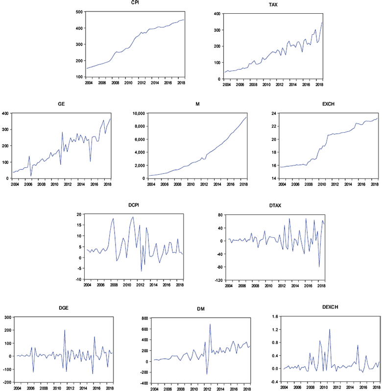
Figure 2. The time series variables at the level and first difference values

4 Result and discussion

Based on the literature of statistics, a unit root is defined as a stochastic trend in a time series. Accordingly, if a time series has a unit root, it will be determined as a systematic pattern that is unpredictable. Some usual testings of statistics (e.g., t, F or the R-squared) cannot have the standard distributions if some of the time series in the function have unit roots (Stock & Watson, 1988). So the unit root test must be employed to test for stationarity in a time series before estimating in the econometric function.

To test the unit root of the variables including the price volatility (CPI), tax revenue (TAX), government expenditure (GE), money supply (M), and exchange rate (EXCH), our paper applies the Augmented Dickey-Fuller (ADF) testing method. The ADF test is chosen because this method allows for less restrictive assumptions for the time series in the function than others. Besides, there are three conditions applied, including (i) with intercept, (ii) with a trend and intercept, and (ii) without a constant for the testing process. The testing results (see Table 2) show that only the Money supply (M) is likely to be stationary at the significance level of 1% (with intercept, and without a constant model), while the remaining variables are non-stationary. However, the testing for the first difference shows that all of these variables are stationary at the significance level of 1%. This result implies that the VAR function will be regressed using the first difference of time-series variables. The unit root test results are presented in Table 2.

Table 2. Result of the Unit root test for the variables

In level
Variable	With intercept	With trend and intercept	Without a constant
Consumer price index (CPI)	-0.941299	-1.307717	2.495925
Tax revenue (TAX)	0.497634	-5.963343***	2.615185
Government expenditure (GE)	-0.295770	-7.743336***	3.127387
Money supply (M)	6.352319***	0.918536	12.13070***
Exchange rate (EXCH)	-0.087253	-1.725585	3.864370
In first difference
Variable	With intercept	With trend and intercept	Without a constant
∆Consumer price index (DCPI)	-4.725130***	-4.753327***	-3.220477***
∆Tax revenue (DTAX)	-3.943663***	-3.970472**	-1.464415*
∆Government expenditure (DGE)	-7.568400***	-7.557685***	-14.97634***
∆Money supply (DM)	-5.454690***	-8.559228***	0.607935
∆Exchange rate (DEXCH)	-6.550527***	-6.494788***	-5.404405***

Note: ***, **, * the rejection of the null hypothesis of unit root at the significance level of 1%, 5%, 10%, respectively. Lag length is 10 periods.
Source: Calculations from the study data

Further, we will test the null hypothesis of no cointegration as opposed to the alternative hypothesis for the variables in the function. Based on our regression strategy in the previous section, the Johansen cointegration test (Johansen, 1988) is employed to examine the possible cointegration vectors between the variables in Equation (1). The testing results indicate that the null hypothesis of no cointegration vector between the variables is rejected at the 1% significance level (see Table 3). The result of the Trace test confirms the existence of at most five cointegration vectors among the variables at the significance of 1%. However, the result of the Max-Eigenvalue test only concludes the existence of at most two cointegration vectors at the significance of 1%. These results imply that there exists a long-term relationship between the consumer price index and the tools of fiscal and monetary policy (including tax, government expenditure, money supply, and exchange rate) in Vietnam over the study period. The result of the Johansen test is summarized in Table 3.

Table 3. Results of the Johansen cointegration test

Rank null hypothesis	r ≤ 0	r ≤ 1	r ≤ 2	r ≤ 3	r ≤ 4
Trace test	170.9*** [0.000]	103.8*** [0.000]	54.02*** [0.000]	29.59*** [0.000]	10.54*** [0.001]
Max-Eigenvalue test	67.05*** [0.000]	49.81*** [0.000]	24.43 [0.016]	19.04 [0.080]	10.54 [0.1001]

Note: *** denotes rejection of the null hypothesis at the significance level of 1%.
Source: Calculations from the study data

After the Johansen test has affirmed the cointegration relationship between the variables in Equation (1), we will analyze the effect of fiscal and monetary policy by the regression of the VAR technique. The next step is the estimated progression to choose an optimal lag for the VAR function. The measurement of policy impulses is performed through the variance decomposition technique and impulse response function. The determination of the optimal lag length for the VAR function is based on a comparison between several reference criteria values. We use five criteria, which include the LR (Sequential modified LR test), PFE (Final prediction error test), AIC (Akaike information criterion test), HQ (Hannan-Quinn information criterion test), and SC (Schwarz information criterion test). According to the results in Table 4, the SC criterion suggests no lag, besides, the LR, FPE, and HQ indicate the optimal four lags, and the AIC confirms the five lags in the VAR function. Because of the limit in the freedom of degrees in our time-series database, the four lags were chosen as the optimal lag length for the VAR equation.

Table 4. Suggestions for the optimal lag length of the VAR function

Lag	LR	FPE	AIC	SC	HQ
0	NA	6.36e+10	39.06551	39.24967*	39.13653
1	57.85788	4.83e+10	38.78606	39.89105	39.21221
2	37.85633	5.18e+10	38.83161	40.85742	39.61288
3	69.95910	2.21e+10	37.91650	40.86315	39.05291
4	42.61261*	1.74e+10*	37.55114	41.41861	39.04267*
5	26.35585	2.13e+10	37.53578*	42.32408	39.38244

Note: * indicates lag order suggested by the criteria. LR: Sequential modified LR test statistic (each test at 5% level). FPE: Final prediction error. AIC: Akaike information criterion. SC: Schwarz information criterion. HQ: Hannan-Quinn information criterion.
Source: Calculations from the study data

In order to test the fitting of the econometric model, the VAR function will be estimated at the four lags, and then we will use the regression result to do some diagnostic tests. First, based on the graph of the unit cycle, we can conclude that the VAR model is appropriate with four lags because all the points are totally located in the unit cycle (see Figure 3). Second, the test for the serial correlation phenomenon will be done by the Lagrange-Multiplier (LM) test. The testing result also confirms there is no serial correlation problem in the VAR model, and it well appropriates for our analysis of the effects of the policies on inflation in the next paragraphs. The Lagrange-Multiplier testing result is represented in Table 5.

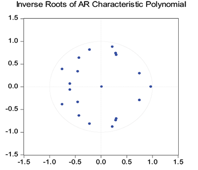
Figure 3. The graph of the Unit cycle

Table 5. Result of the Lagrange Multiplier (LM) test

Lags	LM statistic	Prob
1	23.55545	0.5452
2	23.75974	0.5333
3	50.94705	0.1160
4	31.79087	0.1642
5	23.28462	0.5609

Source: Calculations from the study data

Based on the VAR estimation, the effects of the economic policies on price fluctuations are presented in the following equation. In the VAR function, the fiscal variables are taxation revenue and government expenditure, and the monetary variable includes money supply and exchange rate. The R-squared value is 0.6694, which means 66.94% of the proportion of the variance for the price fluctuation variable that is explained by policy variables in the VAR regression model.

DCPI = 2.963 + 0.545 DCPI(-1) + 0229 DCPI(-2) – 0.383 DCPI(-3)
– 0.062 DCPI(-4) + 0.039 DTAX(-1) + 0.003 DTAX(-2) + 0.039 DTAX(-3)
+ 0.043 DTAX(-4) + 0.002 DGE(-1) + 0.027 DGE(-2) + 0.024 DGE(-3)
– 0.017 DTAX(-4) + 0.009 DM(-1) – 0.001 DM(-2) + 0.005 DM(-3)
– 0.023 DM(-4) + 0.223 DEXCH(-1) – 1.958 DEXCH(-2) + 4.253 DEXCH(-3)
+ 4.234 DEXCH(-4)
R-squared = 0.6694 Adj R-squared = 0.4750

In this part of the study, the variance decomposition is used to analyze the effect of the policies on inflation in the Vietnamese economy. The duration used for the variance decomposition analysis is 10 quarters (2.5 years). The results from variance decomposition report that the tools of fiscal policy only cause 3.13% of the volatility in DCPI in the short run and 24.96% in the long run, however, the tools of monetary policy cause 2.17% of the fluctuation of DCPI in the short run and 23.49% in the long run. Therefore, it could be concluded that the impact of the fiscal policy was stronger than the monetary policy in impulsion of the price volatility over the study period. In summary, the combination of these two policies resulted in 5.30% of the variation in DCPI in the short run and 48.45% in the long run.

Table 6. The variance decomposition results

Variance Decomposition of DCPI
Period	S.E.	DCPI	DTAX	DGE	DM	DEXCH
1	4.073201	100.0000	0.000000	0.000000	0.000000	0.000000
2	4.795218	94.69052	2.355431	0.776656	2.162221	0.015177
3	5.308389	86.93854	3.088692	5.493468	3.364195	1.115103
4	5.535893	80.05566	5.431235	5.792841	5.804127	2.916137
5	6.407950	60.00408	4.208192	19.46650	7.074888	9.246341
6	6.625597	56.34170	3.939857	18.40989	10.59710	10.71144
7	6.745639	54.63937	3.833118	18.46799	10.85933	12.20018
8	6.860045	52.83428	3.893448	20.66339	10.80063	11.80824
9	6.904223	52.60856	3.845250	20.44345	10.74395	12.35878
10	6.977916	51.53976	3.848760	21.11750	10.84007	12.65391

Source: Calculations from the research data

The result also shows that the change in DCPI is affected by the variation of tax revenue of 2.35 % in the short run, and 3.84% in the long run. Moreover, the government expenditure effect on DCPI is 0.77% in the short run and 21.11% in the long run. The result shows that the short-term fluctuation of DCPI made by the money supply is 2.16%, and in the long run it is 10.84%. The exchange rate contributes 0.15% to the volatility of DCPI in the short run, and 12.65% in the long run. Based on the decomposition result, the government expenditure explained the highest proportion in the price fluctuation in Vietnam.

The impact of fiscal and monetary policy on the consumer price index in Vietnam in the research period will be more clearly analyzed using the graphs of impulse response functions. The result of the impulse response functions will add more evidence for the variance decomposition results. We continuously use the period of 10 quarters to analyze the policy impulses in our study. There are four graphs that represent the impact of tools of policies on the consumer price index in the study period. The graph, namely the response of DCPI to DTAX, shows the effect of the tax on CPI. The graph of the response of DCPI to DGE presents the effect of government expenditure on CPI. The impacts of the money supply and exchange rate are shown in the graphs of the response of DM to DCPI as well as the response of DEXCH to DCPI.

First, the effects of tax and money supply on the consumer price index show quite small and faint responses. The tax creates a wave response in the general price level: an increase in tax leads to a slight increase in consumer price index values in the first period, and then the consumer price index returns to balance in the long run. By contrast, the raising of the money supply leads to an increase in the consumer price index in the first period, the consumer price index will decrease and return to balance in the long run. Second, the government expenditure has a remarkable impact on the price fluctuation in which an increase in government expenditure will stimulate consumer price index up to the highest after three quarters, however, the consumer price index is reduced very rapidly and returned to a balanced situation in the long run. Third, the exchange rate has the largest positive effect on price fluctuation in the five quarters, this impact is also significant, after that the general price level slows down and goes to balance in the long run. Obviously, the graphs indicate that the government expenditure and exchange rate have significant impact on price fluctuation in the study period.

The graphs of impulse response function also point out that the effect of fiscal policy is higher than monetary policy. The government expenditure has the highest positive impact on the consumer price index in the third quarter, and the tax revenue has a similar impact at this time. So we can presume that this is a multiplier effect of fiscal policy on inflation. Coming back to the monetary policy, the graphs show that the exchange rate has a strong increasing effect on the consumer price index in the fourth period, however, the money supply has a decreasing impact on the consumer price index at this time. On the other hand, they are opposite effects and will deactivate each other. So this finding means that the effect of monetary policy on the consumer price index is quite small and is not the important reason that induces the fluctuation in the inflation in the study period.

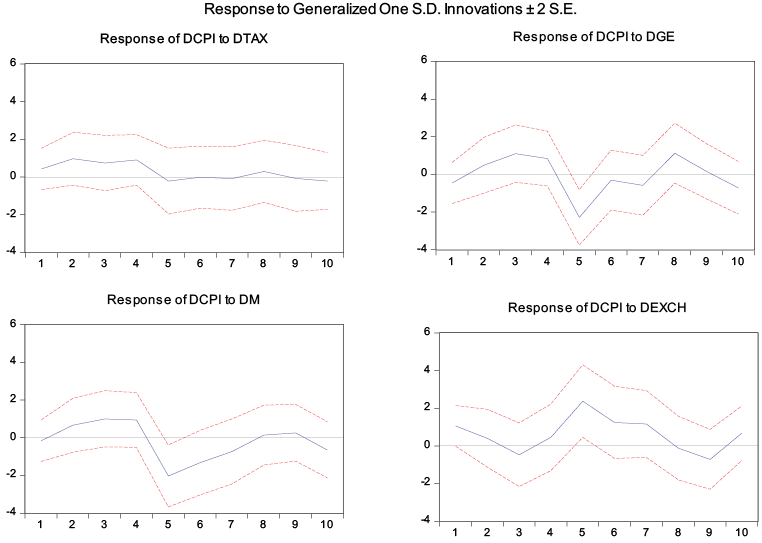
Figure 4. Response functions of the variables from Policy Shocks

According to the impulse response function results, we can conclude that all the primary tools of fiscal and monetary policies contribute to the up-and-down fluctuation on the consumer price index in the research period. It implies that when the government tries to adjust the macro indicators (e.g., supports economic growth), the tools of fiscal and monetary policies are some of the factors that result in the fluctuation of inflation during the last decade in Vietnam. In the four tools of two policies, the government expenditure seems to have the strongest influence on the consumer price index in the study period.

Table 7. Result of the Granger causality test

Hypothesis H₀	Observations	χ² Statistic	P-value
DTAX does not Granger cause DCPI DCPI does not Granger cause DTAX	55	0.61017 2.61091	0.6574 0.0475
DGE does not Granger cause DCPI DCPI does not Granger cause DGE	55	4.52207 0.67217	0.0036 0.6147
DM does not Granger cause DCPI DCPI does not Granger cause DM	55	5.49361 8.03840	0.0011 0.0001
DEXCH does not Granger cause DCPI DCPI does not Granger cause DEXCH	55	2.90103 1.25314	0.0319 0.3020

Source: Calculations from the study data

In order to have a deeper analysis of the real effects of fiscal and monetary policy on price fluctuation in Vietnam, we employ the Granger causality test (Granger, 1988) to identify the causality relationships between the variables in the VAR model. The Chi-squared distribution values of Wald’s test are calculated to conclude the causal relationship between the tools of policies, including the tax, government expenditure, money supply, exchange rate, and the consumer price index. With an application of the VAR model with four lags as the optimal lag length, accordingly, the result of the Granger causality test is reported in Table 7.

There are some interesting findings coming from the testing process. Results of the Granger causality test show some causal relationships between the consumer price index (DCPI) and economic policy variables in the Vietnamese economy. There is a one-way Granger causality from the government expenditure (DGE) to the consumer price index (understood as price fluctuation) as well as a one-way Granger causality from the exchange rate (DEXCH) to consumer price index at the significance level of 5%. The Granger causality test confirms that there is no evidence of the existence of the causal relationships between the tax (DTAX) or the money supply (DM) to the consumer price index in Vietnam in the study period. However, we found a one-way Granger causality from the consumer price index to the tax revenue at the significance level of 5%, and a two-way Granger causality between the consumer price index and the money supply at the significance level of 1%.

The linkage between the graphs of impulse response function and the Granger causality test helps to understand more clearly the effect of fiscal policy and monetary policy on price fluctuation in the case of the Vietnamese economy. All of the investigated results also strongly confirm that the government expenditure (known as a tool of the fiscal policy) and the exchange rate (as a tool of the monetary policy) had robust effects on the consumer price index. Finally, this result could be understood as an assumption that the fiscal policy, as well as the monetary policy, caused inflation in Vietnam in the period of 2004 to 2018.

6 Conclusion

The paper studies the effect of fiscal and monetary policy on price fluctuation in Vietnam, a highlighted emerging economy that has faced some problems regarding galloping inflation over the previous decades. The evidence of these policies in the case of Vietnam is a good reference for policymakers as well as researchers in developing countries, especially emerging economies. Some econometric methods have been employed including the VAR technique, the Johansen cointegration test, and the Granger causality test with a time-series database collected from the first quarter of 2004 to the fourth quarter of 2018.

The policy implications of our paper are multiple. Our findings show that the fiscal policy is more significantly motivating than the monetary policy on inflation in Vietnam. Besides, the impact of government expenditure is the most robust in comparison with other tools, this finding shows that price fluctuation in Vietnam depends on the increase in public expenditure. An increase in government expenditure is the reason that leads to a rise in the consumer price index. The monetary policy affects price fluctuation through the adjustment of the exchange rate but its impact is smaller than the government expenditure of the fiscal policy. Our results conclude that the tools of both policies also contribute to the fluctuation in the consumer price index (of course, the volatility of inflation) in Vietnam in the study period. With the objective of increasing the effectiveness in making and administration policy in order to have moderate inflation in Vietnam in the coming time, the Vietnamese policymakers need to carefully consider the government expenditure (in the fiscal policy) and the exchange rate (in the monetary policy) because our evidence shows that they are the main reasons making increased price fluctuation in Vietnam. The study results also emphasize the price sensitivity to macroeconomic policies in Vietnam, so policymakers at the Central Bank of Vietnam and the Ministry of Finance should be careful using these tools. Furthermore, future studies on inflation may include some macroeconomic variables such as gold price fluctuations (due to Vietnamese people having a habit of storing gold) or cost shocks such as the increase in the price of oil or electricity, which can affect the price fluctuations.

References

Blanchard, O. (2004). Fiscal Dominance and Inflation Targeting: Lessons from Brazil. NBER Working Paper No. 10389.

Bouakez, H., Chihi, F., & Normandin, M. (2014). Measuring the effects of fiscal policy. Journal of Economic Dynamics and Control, 47, 123–151.

Cioran, Z. (2014). Monetary Policy, Inflation and the Causal Relation between the Inflation Rate and Some of the Macroeconomic Variables. Procedia Economics and Finance, 16, 391–401.

Ćorić, T., Šimović, H., & Deskar-Škrbić, M. (2015). Monetary and fiscal policy mix in a small open economy: The case of Croatia. Economic Research-Ekonomska Istrazivanja, 28(1), 407–421.

Dickey, D. A., & Fuller, W. A. (1979). Distribution of the Estimators for Autoregressive Time Series with a Unit Root. Journal of the American Statistical Association, 74(366), 427–431.

Dungey M., & Pagan A. R. (2000), A Structural VAR Model of the Australian Economy. Economic Record, 76, 321–342.

Fan, J., Minford, P., & Ou, Z. (2016). The role of fiscal policy in Britain’s Great Inflation. Economic Modelling, 58, 203–218.

Favero, C. A., & Monacelli, T. (2003). Monetary-Fiscal Mix and Inflation Performance: Evidence from the US. CEPR Discussion Paper No. 3887.

Granger, C. W. J. (1988). Some recent developments in a concept of causality. Journal of Econometrics, 39(1–2), 199–211.

GSO. (2020). Statistics (National accounts) database. Available at http://www.gso.gov.vn/Default_en.aspx? tabid=766 (accessed 22 August 2020).

Hassan, B. (2015). The role of value added tax in the economic growth of Pakistan. International Journal of Public Policy, 11(4–5–6), 204–218.

Hassan, M. S., Islam, F., & Ijaz, M. (2016). Inflation in Pakistan: evidence from ARDL bounds testing approach. International Journal of Management Development, 1(3), 181–195.

Hoa, H. T., Anh, P. T., & Phong, L. T. (2020). Contribution of Manufacturing Strategy to Competitive Performance of Manufacturing Companies: Empirical Evidence from Vietnam. Organizations and Markets in Emerging Economies, 11(2), 482–503.

Hossain, A. A. (2014). Monetary policy, inflation, and inflation volatility in Australia. Journal of Post Keynesian Economics, 36(4), 745–780.

Hossain, A. A. (2015). Inflation volatility, economic growth and monetary policy in Bangladesh. Applied Economics, 47(52), 5667–5688.

Jalil, A., Tariq, R., & Bibi, N. (2014). Fiscal deficit and inflation: New evidences from Pakistan using a bounds testing approach. Economic Modelling, 37, 120–126.

Johansen, S. (1988). Statistical Analysis of Cointegration Vectors. Journal of Economic Dynamics and Control, 12(2–3), 231–254.

Lapukeni, A. F. (2015). The impact of financial inclusion on monetary policy effectiveness: T he case of Malawi. International Journal of Monetary Economics and Finance, 8(4), 360–384.

Mankiw, N. G. (2009). Macroeconomics, 7^th Edition. New York, USA: Worth Publishers.

Martínez-López, D. (2017). How does fiscal reform affect the elasticity of income tax revenues? The case of Spain, 2003–2008. International Journal of Public Policy, 13(6), 337–357.

McGregor, H. (2011). Jim O’Neill Game Changer. Brunswick Review, 4 (Summer), 27–29.

Mikek, P. (2008). Alternative monetary policies and fiscal regime in new EU members. Economic Systems, 32(4), 335–353.

Tkacevs, O. (2006). The Impact of Fiscal Policy on Prices: Does the Fiscal Theory of Price Level Matter in Latvia. Baltic Journal of Economics, 6(1), 23–36.

Owoye, O., & Onafowora, O. A. (1994). The relative importance of monetary and fiscal policies in selected African countries. Applied Economics, 26(11), 1083–1091.

Pagan, A. R., & Pesaran, M. H. (2008). On the Econometric Analysis of Structural Systems with Permanent and Transitory Shocks and Exogenous Variables. Journal of Economic Dynamics and Control, 32(10), 3376–3395.

Stock, J. H., & Watson, M. W. (1988). Testing for common trends. Journal of the American Statistical Association, 83, 1097–1107.

Semmler, W., & Zhang, W. (2004). Monetary and Fiscal Policy Interactions in the Euro Area. Empirica, 31(2–3), 205–227.

Tekin-Koru, A., & Özmen, E. (2003). Budget deficits, money growth and inflation: The Turkish evidence. Applied Economics, 35(5), 591–596.

Traum, N., & Yang, S. S. (2010). Monetary and fiscal policy interactions in the post-war USA. Working Paper No. 10/243, IMF, USA.

Tung, L. T. (2020). Factors affecting labour productivity of employee in an Asian emerging market: evidence in Vietnamese retail sector. International Journal of Business and Globalisation, 24(4), 513–528.

Vargas, J. M. F. (2012). Money growth and inflation: Evidence from post-inflation Bolivia. International Journal of Economic Policy in Emerging Economies, 5(4), 353–366.

Wilson, D., & Stupnytska, A. (2007). The N-11: More Than an Acronym. Global Economics Paper No: 153, Goldman Sachs.

World Bank (2020). The World Bank in Vietnam: Overview. Available at: http://www.worldbank.org/en/country/vietnam/overview (accessed 11 October 2020)

World Bank (2021). World Bank Open Data. Available at: https://data.worldbank.org/indicator (accessed 22 January 2021)