Organizations and Markets in Emerging Economies ISSN 2029-4581 eISSN 2345-0037
2022, vol. 13, no. 1(25), pp. 238–259 DOI: https://doi.org/10.15388/omee.2022.13.78

Analyzing Exchange Market Pressure Dynamics with Markov Regime Switching: The Case of Turkey

Ali İlhan (corresponding author)
Tekirdağ Namık Kemal University, Faculty of Economics and Administrative Sciences,
Department of Economics, Turkey
ailhan@nku.edu.tr
https://orcid.org/0000-0001-6201-5353

Coşkun Akdeniz
Tekirdağ Namık Kemal University, Faculty of Economics and Administrative Sciences,
Department of Economics, Turkey
cakdeniz@nku.edu.tr
https://orcid.org/0000-0002-3973-754X

Metin Özdemir
Burs Uludağ University, Faculty of Economics and Administrative Sciences,
Department of Economics, Turkey
mozdemir@uludag.edu.tr
https://orcid.org/0000-0002-3944-4018

Abstract. This study analyzes the dynamics of exchange market pressure in Turkey by employing the Markov regime switching model for the period from January 2006 to December 2019. Our findings show that there are two regimes in the foreign exchange market, characterized as low- and high-pressure periods. The domination of the high-pressure regime in the sample period indicates that depreciation pressure prevails in the Turkish foreign exchange market. During this regime, the pressure is aggravated by the rising inflation, credit growth, and VIX, and the falling of short-term external debt. Thus, in the presence of capital flows, the preferences of policy authorities regarding price stability and growth determine the course of the pressure. When these policy choices favor credit-driven growth, depreciation pressure in the foreign exchange market is exacerbated through the current account deficit.

Keywords: capital flows, exchange rate, exchange market pressure, macroeconomic fundamentals, managed floating exchange rate regime, Markov regime switching, Turkey

Received: 18/8/2021. Accepted: 25/11/2021
Copyright © 2022 Ali İlhan, Coşkun Akdeniz, Metin Özdemir. Published by Vilnius University Press. This is an Open Access article distributed under the terms of the Creative Commons Attribution Licence, which permits unrestricted use, distribution, and reproduction in any medium, provided the original author and source are credited.

1. Introduction

Following the financial crises experienced under the fixed exchange rate regime during the 1990s, several emerging market economies (EMEs) adopted inflation targeting and a flexible exchange rate regime (Bernanke et al., 1999). While the latter acts as a shock absorber (Edwards & Yeyati, 2005) against the shocks that hit the economy, the monetary policy aims at price stability. However, inflation targeting does not isolate economies from all external shocks (Siklos, 2018), although it contributes to exchange rate stability (Rose, 2007; Lin, 2010).

Many EMEs have intervened in the foreign exchange market despite a clear commitment to floating exchange rates (Ilzetzki et al., 2019). The fear of floating (Calvo & Reinhart, 2002) due to various factors, such as currency mismatches in balance sheets and the high exchange rate pass-through (Ostry et al., 2012), and the need to accumulate reserves against shocks (Aizenman & Hutchison, 2012) forces policy authorities to intervene in their foreign exchange market. Ghosh et al. (2016) argue that most emerging market central banks have an implicit comfort zone for smoothing large and abrupt exchange rate movements, even if they do not set an exchange rate target.

The global financial crisis (GFC) showed that high exchange rate volatility may lead to negative consequences for financial stability beyond price stability. Unconventional monetary policies implemented by advanced economies, mainly the Federal Reserve, including large asset purchases and near-zero policy rates, have accelerated capital inflows to EMEs (Dell’Ariccia et al., 2018). The abundance of global liquidity and monetary spillovers reveals the policy interconnectedness between advanced economies and EMEs, even under a flexible exchange rate regime¹ (Taylor, 2013; Edwards, 2018). Rey (2013) also claims that the global financial cycle in capital flows, credit growth and asset prices exposes EMEs to new shocks. Due to global integration, the global financial cycle constrains domestic monetary policies; therefore, a floating exchange rate is not enough to insulate the domestic economy.

Exchange rate shocks triggered by changes in global liquidity conditions can cause conflicts between policy objectives (Obstfeld, 2015). In this respect, the concerns of high volatility in exchange rates arise over the international dimension of the risk-taking (financial) channel of monetary policy (Bruno & Shin, 2015; Georgiadis & Zhu, 2019). An exchange rate appreciated by capital flows may lead to credit expansion and a rise in aggregate demand by reducing the banking sector’s external costs. If the financial channel works effectively, there may be a conflict between price stability and growth. Potential financial vulnerabilities stemming from credit expansion may cause financial instability due to a sudden reversal in capital flows (Agénor et al., 2020). Hence, EMEs actively participated in the foreign exchange market to strengthen their international reserves against the risk of a sudden stop and to reduce appreciation pressure on their domestic currency during accelerated capital inflows. Furthermore, when capital outflows increase, they step into the foreign exchange market to limit the macro-financial risks from depreciation pressures (Blanchard et al., 2015). Therefore, managed floating has become the standard for many EMEs in the post-crisis era, whether they have adopted inflation targeting or not² (Frankel, 2019).

Recent literature has shown that reductions in the exchange rate pass-through (Mihaljek & Klau, 2008) and inflation targeting help stabilize exchange rate pressures (Feldkircher et al., 2014; Soe & Kakinaka, 2018). Contrary to systemic crisis periods when sudden stops cause capital outflows, monetary spillovers due to unconventional policies have increased interest in the relationship between financial stability and exchange rate pressure in EMEs (Mohanty, 2014; Aizenman & Binici, 2016; Ozcelebi, 2020).

The exchange rate volatility plays a crucial role in EME policy choices. To explain and control the effects of exchange rate volatility, it is necessary to know the dynamics of the exchange market and the factors that put pressure on the exchange rate (Ozcelebi, 2019). In intermediate regimes where policy authorities intervene in the foreign exchange market, the exchange rate cannot fully capture the pressure. This can be achieved using the exchange market pressure (EMP) index, which includes exchange rate changes and foreign exchange interventions (Klaassen & Jager, 2011; Olanipekun et al., 2019). The EMP index is an important tool for understanding developments in the foreign exchange market under different exchange rate regimes and for developing appropriate policy responses (Tanner, 2000, 2002).

Turkey is one of the EMEs exposed to the macro-financial risks associated with capital inflows in the post-crisis era. Accelerated credit growth and the appreciating Turkish Lira (TL), the increasing weight of portfolio inflows for financing a widening current account deficit have led to a need for a flexible policy framework towards changes in global risk appetite. Accordingly, in November 2010, the Central Bank of the Republic of Turkey (CBRT) designed a framework called the new policy mix. One of its intermediate targets was slowing down short-term capital inflows, while the exchange rate was one of the intermediate variables. Unconventional instruments, such as the reserve option mechanism and the asymmetric interest rate corridor, were employed to ensure exchange rate stability and achieve effective reserve management against sudden stop risks (Kara, 2013).

The high level and persistence of the current account deficit in the Turkish economy threatens the sustainability of its growth. Dependence on short-term capital in-flows to finance growth makes the economy vulnerable to global financial conditions and external shocks. The risk of financial instability arising from external dominance puts pressure on the foreign exchange market. Therefore this paper aims to analyze the dynamics of EMP in Turkey. To this end, we calculate the EMP index in Turkey and analyze its determinants during different periods. More specifically, a Markov regime switching (MS) model is employed to estimate EMP dynamics in Turkey for the period from January 2006 to December 2019.

Many studies have demonstrated the time-varying relationship between exchange rates and macroeconomic fundamentals (Frömmel et al., 2005; Junttila & Korhonen, 2011; Yuan 2011; Wu, 2015; Beckmann et al., 2018). MS models define different states of regimes and allow us to analyze the asymmetric behaviors of variables conditional on the regimes (Baharumshah et al., 2017). Kumah (2011) showed that MS models can help to understand the factors affecting low and high foreign exchange market pressures. Therefore, we investigate the determinants of EMP by employing the Markov Regime Switching Intercept Autoregressive Heteroscedasticity (MSIAH) model.

This study analyzes the EMP dynamics in Turkey with a time series in a nonlinear manner for a period covering before and after the GFC. Our study contributes to the literature in the following ways. First, our findings demonstrate that there are two different regimes in the Turkish foreign exchange market and determinants of EMP that exhibit asymmetrical behavior in terms of sign and magnitude. This supports claims about the nonlinear nature of the EMP and its time-varying relationship with macroeconomic factors (Kumah, 2011). Second, in the high-pressure regime, which dominates the sample period, an increase in inflation, credit growth, and the volatility index (VIX), and a decrease in short-term external debt exacerbate pressure in Turkey. This provides supporting empirical evidence for the importance of macroeconomic fundamentals, and capital flows in explaining the EMP in EMEs (Aizenman et al., 2012; Tan et al., 2020).

The rest of the paper is organized as follows. The next section describes the EMP index and the empirical literature on EMP. The third section introduces the estimated model and employed variables. The fourth section explains the MS model, and the fifth section reports the empirical findings. The following section concludes the paper.

2. Literature Review

2.1 Exchange Market Pressure Index

The EMP index, developed by Girton and Roper (1977), obtained by summing the change in the exchange rate and international reserves, is described as a variable that reflects the level of intervention required to achieve the exchange rate target. The Girton and Roper (1977) model, based on a monetary approach to ensure the balance of payments, assigns equal weights to components of the EMP index. In contrast, Roper and Turnovsky (1980) replaced the monetary model with a small open economy model by differentiating the equal weights assigned to the original index components. Weymark (1995) suggested a model-independent definition to formalize the EMP index. That is, EMP measures the exchange rate changes that will eliminate excessive demand for a currency if there is no intervention in the exchange market. If the domestic currency fluctuates freely, the pressure in the foreign exchange market can be observed directly through exchange rate changes. In intermediate regimes, such as managed floating exchange rate changes, foreign exchange intervention measures should also be considered. To this end, Weymark (1995) put forward a more general formula that transforms the previous models into special cases and included an elasticity coefficient in the EMP calculation that converts observed intervention changes into exchange rate units.

Based on criticisms of model-dependent EMP measurements, alternative model-independent approaches have been developed. Unlike Weymark’s (1995) model-dependent method, Eichengreen et al. (1996) calculated the index component weights independently from the model. They aimed to equalize the volatility of the components by using sample variances in the weight calculation and to eliminate the distortion effects of high volatility components on the index. They also added an interest rate component to the index, given that interest rate hikes are a policy option against speculative attacks.

Another discussion concerning the EMP index calculation is the form of the interest rate component. Van Horen et al. (2006) and Mody and Taylor (2007) considered the first difference of the domestic interest rate in their calculations. Eichengreen et al. (1996), Pentecost et al. (2001), and Hegerty (2009) employed the change in the interest rate differential. On the other hand, Klaassen and Jager (2011) opposed the inclusion of the traditional forms of interest component by proposing a definition-consistent EMP measurement. They suggested that the interest rate differential should be taken in level form by subtracting the counterfactual interest rate, in which the interest rate of a country lacks an exchange rate target, from the domestic interest rate.³

2.2 Relevant Empirical Literature

Early EMP studies focused on the macroeconomic variables associated with the exchange rate and the implications of monetary policy. Pentecost et al. (2001) investigated the determinants of EMP on European currencies covering the period from 1980 to 1994. They concluded that the budget deficit, current account deficit, real depreciation, long-term interest rate, and differential money growth explain the EMP in five member countries of the European Exchange Rate Mechanism. Tanner (2002) analyzed the relationship between EMP and monetary policy in 32 EMEs. He argued that pressures were dampened by tightening the monetary policy stance, as reflected by domestic credit growth and the nominal interest rate differential. Gochoco-Bautista and Bautista (2005) examined the relationship between EMP and monetary policy in the Philippines from January 1990 to April 2000, finding that the rising interest rate differential and the slowdown in credit growth decreases EMP in normal times, whereas the impact of the rise in the interest rate differential has a positive impact on EMP during crises.

Feldkircher et al. (2014) used a wide panel of 149 countries and 58 indicators to examine the leading indicators explaining EMP during the GFC. They found that price stability is a crucial determinant of the exchange rate pressure. In the pre-crisis period, the increase in domestic savings in countries with low inflation reduced the pressure. Hegerty (2014) explored the effects of macroeconomic variables, external factors, and commodity prices on the EMP in four Latin American countries for February 1992 to November 2010. Inflation was the key determinant of EMP, whereas increasing public debt and domestic credit growth had a relatively small effect. Panday (2015) analyzed the interaction between EMP and monetary policy in Nepal from 1975 to 2009. While the effect of the money multiplier and domestic credit was positive, output growth decreased EMP.

The interaction between capital flows and exchange rates and financial risk factors due to global financial integration and monetary spillovers (Plantin & Shin, 2016; Kalemli-Özcan, 2019) has led to the investigation of the relationship between the EMP index and the vulnerabilities of EMEs. Aizenman et al. (2012) examined the determinants of EMP in 27 EMEs for the 2000s. They demonstrated that the declining income growth, increasing domestic credit, rising inflation, deteriorating trade balance, net portfolio debt outflows, and decreased gross short-term external debt increased EMP during the Great Moderation. While income, domestic credit, net portfolio debt outflows, and gross short-term external debt remained the determinants of EMP during the GFC, the coefficient of gross short-term external debt increased considerably at the beginning of the crisis. Investigating 2000Q1 – 2014Q3 for 50 OECD and EMEs, Aizenman and Binici (2016) concluded that external factors play a crucial role in EMP, while short-term capital flows have significant effects on the EMP in EMEs. Tan et al. (2020) showed that credit and portfolio flows are significant indicators of both extreme negative and positive EMP episodes in EMEs. Ozcelebi (2020) demonstrated that the increase in the developed country’s financial stress index raises the pressure on the EMP index in EMEs.

The studies which analyzed the EMP dynamics in Turkey can be classified into two groups. The first group used the EMP index as a dependent crisis variable to explain the determinants of currency crisis episodes. Çeşmeci and Önder (2008) investigated the determinants of currency crises for February 1992 – October 2004 with three different methods. With all the three methods, public sector variables, the real sector confidence index, and the money market pressure index were found to be significant indicators of currency crises. Feridun (2008) found that the 1994 and 2000–2001 currency crises are linked with fiscal imbalances, banking sector fragilities, global liquidity conditions, and capital outflows. Ari and Cergibozan (2018) analyzed currency crisis episodes in Turkey between 1990 and 2014. They demonstrated that the ratio of bank foreign deposits to total deposits, portfolio investments, and the inflation rate were the key determinants of currency crises, measured by various speculative pressure indices.

The second group of studies addressed the EMP beyond currency crisis episodes. Feridun (2009), who examined the macroeconomic determinants of EMP in Turkey for August 1989 – August 2006, found a causal relationship between banking sector fragility, M2 to international reserves, an overvalued real exchange rate, and EMP. Feridun (2010) also analyzed the relationship between capital reversals and EMP and demonstrated both a short- and long-run causality from capital reversals to EMP. Katircioglu and Feridun (2011) found a unidirectional causality from domestic credits, international reserves, real money supply, budget, and current account balance to EMP. Siklar and Akca (2020) investigated the relationship between the monetary policy and EMP in Turkey, covering the period from January 2002 to December 2018. They found bidirectional causality between the interest rate differential and EMP and unidirectional causality from domestic credit to EMP. However, the interest rate differential and domestic credit had a significant positive effect on EMP. To deepen the knowledge obtained in previous research, this study investigates whether macroeconomic fundamentals and capital flows affect the EMP in Turkey.

3. Model and Data

Eichengreen et al. (1996) argued theoretically that the EMP index should be derived from a structural exchange rate determination model. However, such models have weak explanatory power at short- and medium-term horizons. Hence, in the absence of an empirically valid macroeconomic model, the exchange rate market pressure can be analyzed with an ad hoc approach.

Exchange rate and reserve changes as well as the interest rate differential, which is compatible with the managed floating of EMEs, are also used in the EMP calculations in the literature. In times of depreciation, the use of the interest rate to ensure the stability of the exchange rate in Turkey due to the fear of financial stability (Özdemir, 2020) necessitates including the interest rate differential in the EMP calculations. Thus, similar to the index employed by Aizenman and Binici (2016), a standardized index of three components is used in this study.

(1)

where empi_t represents the exchange market pressure index; μ and σ denote the mean and standard deviation of the variables, respectively; ∆e_t and ∆ir_t stand for the annual percentage changes in the nominal exchange rate and international reserves, respectively.⁴ While the nominal exchange rate is the USD/TL rate, gold reserves are excluded from the international reserves. ∇i_t reflects the nominal interest rate differential, calculated by subtracting US interest rates from Turkish interest rates based on overnight interbank interest rates in both countries.

We constructed the model for estimating the determinants of EMP in Turkey by considering the relevant empirical literature. The following variables are included in the model as potential determinants of EMP: domestic income and inflation, which are used in monetary models to explain exchange rate fluctuations (Civcir, 2003), domestic credit as an indicator of monetary policy stance (Tanner, 2000, 2002), short-term external debt stock that reflects capital flow implications (Aizenman et al., 2012), and the VIX that indicates the global risk appetite (Gevorkyan, 2019). The model estimated for January 2006 – December 2019 is specified as follows:

(2)

where y_t indicates the industrial production index, which is the proxy for domestic income; inf_t reflects the consumer price index; crdt_t denotes the total credit volume of the banking sector; std_t represents the short-term external debt stock; and vix_t shows the volatility index. The daily frequency of VIX is converted into monthly frequency based on the last observation in that month. While α denotes the constant term, ε_t indicates the error term. The series showing a seasonal effect are seasonally adjusted employing the Census X-13 method. All explanatory variables are used as annual percentage changes and standardized to eliminate level differences between the series.

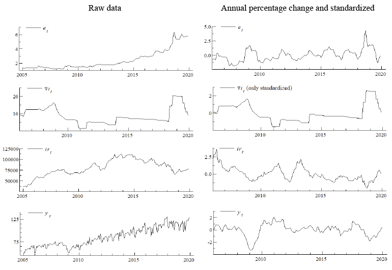
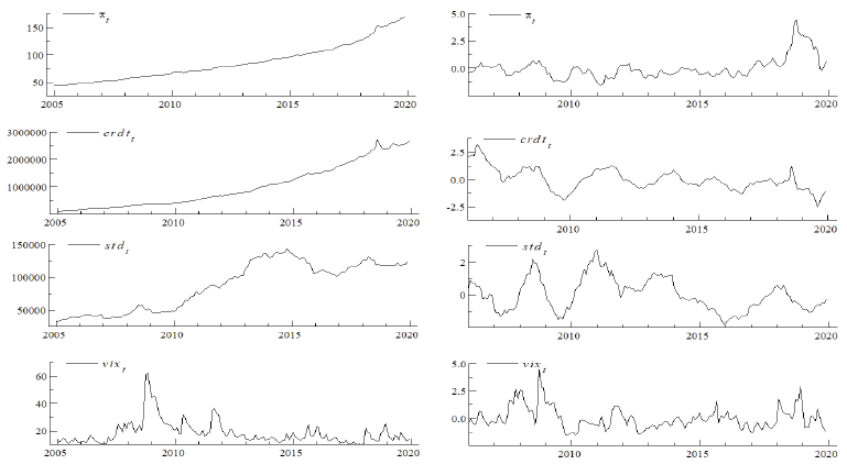
The series used in the study were obtained from various databases. Exchange rates, interest rates, the industrial production index (2010=100), and the consumer price index (2010=100) were retrieved from OECD Main Economic Indicators. International reserves were obtained from the IMF International Financial Statistics. The total credit volume of the banking sector was imported from the Banking Regulation and Supervision Authority. Short-term external debt stock was retrieved from the CBRT. The volatility index was obtained from the Chicago Board Options Exchange. Time series plots of the data are shown in Appendix A.

4. Methodology

Various events may cause permanent or temporary changes in a time series. The models that consider parameter variation should be used in the presence of these changes. To this end, MS models are employed to reveal these changes depending on the state variable (Yağcıbaşı & Yıldırım, 2019).

MS models were popularized by Hamilton (1989), who used them for macroeconomic time series. In MS models, because regime switching does not result from a deterministic process, it can be defined as a random variable. Thus, regime switching is defined by the unobservable random variable s_t, called the state or regime variable. Regimes are determined according to the values taken by s_t. The simplest time series model for this kind of discrete-valued random variable is the Markov chain (Hamilton, 1994).

It is assumed that s_t takes only an integer value {1, 2, …, N}. The Nth order Markov chain, which reveals the probability of s_t being equal to a certain value of j through its recent value, is expressed in the following equation:

(3)

Here, the transition probabilities of state i followed by state j are represented by p_ij. The transition matrix P, for NxN dimensions is defined as follows under the assumption of p_i1 + p_i2 + ... p_iN =1 (Hamilton, 1994):

(4)

In the empirical analysis, some parameters proceed on the state, while the rest of the parameters can be regime invariant components of the Markov chain. Krolzig (1997) identifies the regime-dependent parameters with the general MS(M). Among the MS models, we employed the MSIAH model as this considers full parameter shifts and also allows the variance of the residuals to change across states (Çatık & Önder, 2011).

The MS model is estimated by the maximum likelihood estimator based on the expectation-maximization (EM) algorithm. According to this algorithm, the observed variables are bound up with unobservable stochastic variables. The EM algorithm iteration has two steps: expectation and maximization, respectively. The first step is based on the filtering and smoothing algorithms employing an estimated parameter instead of the unknown true parameter. In this way, smoothed probabilities can be estimated from the unobserved states. In the second step, the estimated parameter is obtained by using the first-order conditions linked with the likelihood function to substitute conditional regime probabilities with smoothed probabilities. The new parameter of the smoothed and filtered probabilities is updated in the following expectation step. Thus, each step raises the likelihood value⁵ (Krolzig, 1998).

The model presented in Equation (2) in a linear form can be re-written with the two regime MSIAH model:

(5)

In this model, s_t represents the state variable, which takes an integer value 1 or 2. If s_t = 1, the low-pressure regime is valid in the foreign exchange market. If s_t = 2, then the high-pressure regime prevails. All the estimated coefficients of the parameters are highly dependent on s_t .

5. Empirical Findings

We analyzed the EMP dynamics in Turkey for two different regimes. Regime 1 represents low-pressure periods in the foreign exchange market, whereas Regime 2 represents high-pressure periods. Table 1 displays the properties and transition matrix of these regimes.

Table 1
Regime Properties and Transition Matrix

Regime Properties
	Observation		Probability		Duration
Regime 1	48.0		0.171		24.47
Regime 2	120.0		0.828		118.01
Transition Matrix
		Regime 1		Regime 2
Regime 1		0.9591		0.0409
Regime 2		0.0085		0.9915

Source: Authors’ calculations

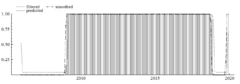
The high-pressure regime covers around three-quarters of the sample period with higher probability and longer duration. The transition matrix shows that the probability of switching from the low- to the high-pressure regime is higher at 4.09% than vice versa at 0.85%. Figures 1–3 show the EMP index calculated for Turkey based on Equation (1) and regime probabilities.

Figure 1
EMP Index

 

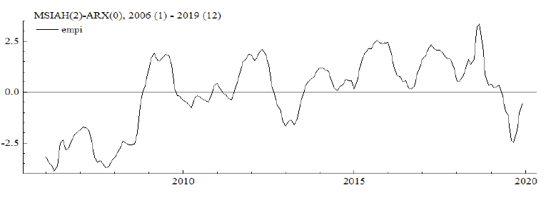
Figure 2
Regime 1 Probabilities

 

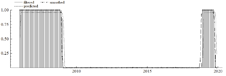
Figure 3
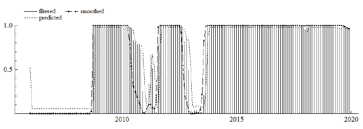
Regime 2 Probabilities

 

Source: Authors’ calculations

Figure 2 shows that the low-pressure regime prevailed in Turkey prior to the GFC. The low-pressure reflects a period of large capital inflows to the Turkish economy due to the declining risk premium. When the effects of the GFC emerged in the third quarter of 2008, the foreign exchange market shifted to the high-pressure regime, as indicated in Figure 3. During this period, when the implications of the GFC and the Euro debt crisis were felt severely, the CBRT adopted the exchange rate as one of its intermediate variables under its new policy mix. As shown in Figure 1, the decrease in EMP since the end of 2012 reflects the efforts to reduce the sudden stop risk with both macroprudential tools and traditional policy instruments. However, the high-pressure regime persisted despite the decline in pressure.

In May 2013, the taper talk (Bernanke, 2013) that strengthened tighter monetary policy expectations led to notable capital flight from Turkey, similar to many EMEs. The sharp depreciation in the exchange rate after the taper talk confirms that the increase in pressure became clear after the second half of 2013. During this period, the exchange rate stability achieved by higher interest rates and the use of international reserves was interrupted by a series of domestic and external shocks. After the exchange rate shock of August 2018, EMP reached its peak in the sample period. After this date, the low-regime prevailed for a short time due to the decrease in pressure.

Before proceeding to the estimation results regarding the determinants of EMP, it is necessary to review the findings of the linearity test. The validity of the linear model was analyzed with the likelihood ratio (LR) linearity test, which shows that the linear model is not valid. Furthermore, the comparison of the Akaike information criterion (AIC) and log-likelihood values of the nonlinear and linear models confirms the two-regime MSIAH model (Çatık & Önder, 2011; Baharumshah et al., 2017).

Table 2
Estimation Results

Regime 1 (Std. Error: 0.511)
Variable	Coefficient	Standard Error	t-value
α	-2.822***	0.133	-21.199
yt	-0.930***	0.178	-5.221
πt	0.623***	0.125	4.952
crdtt	0.219**	0.089	2.454
stdt	-0.337***	0.110	-3.050
vixt	-0.003	0.007	-0.050
Regime 2 (Std. Error: 0.615)
Variable	Coefficient	Standard Error	t-value
α	1.211***	0.065	18.558
yt	-0.107	0.079	-1.359
πt	0.262***	0.073	3.589
crdtt	1.068***	0.140	7.625
stdt	-0.887***	0.081	-10.880
vixt	0.226**	0.096	2.354

 

LR Linearity Test: 316.359	Chi (7) = (0.000)***	Chi (9) = (0.000)***
	Log-likelihood	AIC
Nonlinear model	-160.933	2.106
Linear model	-319.113	3.882

Note. ***, **, and * indicate significance at 1%, 5%, and 10%, respectively.
Source: Authors’ calculations

The coefficients of Regime 1 reveal that all explanatory variables except VIX are statistically significant. During periods of low-pressure, rising inflation and credit growth increase the pressure, whereas increasing domestic income and short-term external debt ease the pressure. VIX has no significant impact on EMP. On the other hand, the coefficients of Regime 2 indicate that the effect of VIX becomes significant, whereas the effect of domestic income becomes insignificant. In the high-pressure regime, the increasing inflation, acceleration of credit growth, the rising VIX, and the fall of short-term external debt strengthen the pressure. Furthermore, the magnitude of variables, which are significant in both regimes, differ. In the high-pressure regime, the coefficient of credit and short-term external debt is higher, whereas inflation is lower. The high coefficients of credit growth and short-term external debt compared to other determinants illustrate their key effect on EMP in the high-pressure regime.

Domestic income and inflation are among the explanatory variables of monetary models established to understand exchange rate movements. In the monetary exchange rate models, an increase in the expected domestic price level and a decrease in domestic income are expected to reduce demand for the domestic currency, thereby increasing depreciatory pressure (Frankel, 1979). Table 2 shows that the effect of domestic income on EMP is negative in the low-pressure regime, while the effect is insignificant in the high-pressure regime. According to the Mundell–Fleming model, increasing real income worsens the trade balance through the import channel and requires a rise in the nominal exchange rate to restore equilibrium (Civcir, 2003). The insignificant effect of domestic income in the high-pressure regime may be attributed to the negative effect of the domestic income on the nominal exchange rate disappearing with the trade balance effect. On the other hand, inflation has a significant and positive impact on EMP in both regimes. This finding highlights the importance of price stability for EMP.

However, according to Tanner (2002), the interest rate is an ex-ante indicator that reflects the intentions of monetary authorities, whereas domestic credit indicates the ex-post monetary policy stance. An expansionary monetary policy shock that manifests itself in increasing credit growth causes a depreciation of the domestic currency under a flexible exchange rate regime but a loss of international reserves under a fixed exchange rate regime (Gochoco-Bautista & Bautista, 2005; Samba, 2018). The positive sign of domestic credit growth in the high-pressure regime confirms that expansionary policies shaped by the economic growth preferences of policy authorities increase the pressures on the exchange market.

Aizenman et al. (2012) suggest that gross short-term external debt reflects “hot money” flows. In times of capital outflows and deleveraging, foreign currency demand increases. EMEs accommodate the deleveraging by using their international reserves due to the balance sheet implications rather than allowing the exchange rate to depreciate. As displayed in Table 2, the fall of short-term external debt increases EMP in both regimes. This illustrates the critical role of capital flows for the EMP dynamics and monetary policy in Turkey (Özatay, 2016).

The carry trade literature asserts a relationship between carry trade flows and VIX (Rey, 2013). Forbes and Warnock (2012) also demonstrated that gross capital inflows are linked with decreasing VIX. Thus, when the course of VIX is high and volatile, EMP is expected to increase (Gevorkyan, 2019). Similarly, our findings show that VIX has a significant and positive impact on EMP in the high-pressure regime. In other words, tightening global liquidity conditions strengthens the pressure in the foreign exchange market.

We performed a robustness check by changing the EMP index and the model. EMP was recalculated by subtracting the interest component from Equation (1) and adding the interest rate differential to the right side of Equation (2). The regime probabilities and the estimated coefficients of the high-pressure regime remained largely consistent with the original findings.⁶ Moreover, the effect of interest rate differential on EMP is insignificant in the low-pressure regime, while the effect is negative in the high-pressure regime. This implies that the interest rate determines EMP only in the high-pressure regime.

6. Conclusion

Exchange rate fluctuations can have distorting effects on macroeconomic stability in EMEs. Low credibility and vulnerabilities may lead to long-lasting pressure on their currencies. Despite being floaters, they step into the foreign exchange market due to fear of floating and sudden stop risks. In these countries, identifying the pressure in the foreign exchange market and its determinants is important for developing appropriate policy responses. To this end, this study investigated the EMP dynamics in Turkey using the MS model for January 2006 – December 2019.

Our findings show that there are two regimes in the Turkish foreign exchange market, characterized as low- and high-pressure periods. The domination of the high-pressure regime in the sample period indicates that depreciation pressure prevails in the Turkish foreign exchange market. The high-pressure regime, which switched with the GFC, persisted for a long time due to the taper tantrum. During this period, the pressure was exacerbated by a series of domestic and external shocks.

The estimation results show that the behavior of some variables is asymmetric. The negative effect of domestic income on EMP is significant in the low-pressure regime, whereas VIX has a significant effect in the high-pressure regime. Moreover, the magnitudes of variables, which are significant in both regimes, differ. In the high-pressure regime, the coefficient of credit and short-term external debt is higher, whereas inflation is lower. This suggests that credit growth and capital flows become more important in determining pressure in times of depreciation.

The findings demonstrate that inflation, credit growth, short-term external debt, and VIX play determining roles in the high-pressure regime. A rise in inflation, acceleration of credit growth, the increasing VIX, and decreasing short-term external debt strengthen pressure in the Turkish foreign exchange market. Thus, in the presence of capital flows, the preferences of policy authorities regarding price stability and growth determine the course of the pressure. When these policy choices favor credit-driven growth, the depreciation pressure in the foreign exchange market is exacerbated through the current account deficit.

References

Agénor, P-R., Jackson, T. P., & Pereira da Silva, L. (2020). Foreign Exchange Intervention and Financial Stability. BIS Working Papers No. 889.

Aizenman, J., & Hutchison, M. M. (2012). Exchange market pressure and absorption by international reserves: Emerging markets and fear of reserve loss during the 2008–2009 crisis. Journal of International Money and Finance, 31(5), 1076–1091. https://doi.org/10.1016/j.jimonfin.2011.12.011

Aizenman, J., Lee, J., & Sushko, V. (2012). From the Great Moderation to the Global Crisis: Exchange Market Pressure in the 2000s. Open Economies Review, 23(4), 597-621. https://doi.org/10.1007/s11079-011-9228-y

Aizenman, J., & Binici, M. (2016). Exchange market pressure in OECD and emerging economies: Domestic vs. external factors and capital flows in the old and new normal. Journal of International Money and Finance, 66, 65–87. https://doi.org/10.1016/j.jimonfin.2015.12.008

Ari, A., & Cergibozan, R. (2018). Currency crises in Turkey: An empirical assessment. Research in International Business and Finance, 46, 281–293. https://doi.org/10.1016/j.ribaf.2018.04.001

Baharumshah, A. Z., Soon, S-V., & Wohar, M. E. (2017). Markov-switching analysis of exchange rate pass-through: Perspective from Asian countries. International Review of Economics and Finance, 51, 245–257. https://doi.org/10.1016/j.iref.2017.05.009

Beckmann, J., Glycopantis, D., & Pilbeam, K. (2018). The dollar-euro exchange rate and monetary fundamentals. Empirical Economics, 54(4), 1389–1410. https://doi.org/10.1007/s00181-017-1335-1

Bernanke, B. S., Laubach, T., Mishkin, F. S., & Posen, A. S. (1999). Inflation Targeting: Lessons from the International Experience. Princeton: Princeton University Press.

Bernanke, B. S. (2013). The Economic Outlook. Available at: https://www.federalreserve.gov/newsevents/testimony/bernanke20130522a.htm (accessed 14 April 2021)

Blanchard, O., Dell’Ariccia, G., & Mauro, P. (2010). Rethinking Macroeconomic Policy. Journal of Money, Credit and Banking, 42(s1), 199–215. https://doi.org/10.1111/j.1538-4616.2010.00334.x

Blanchard, O., Adler, G., & de Carvalho Filho, I. (2015). Can Foreign Exchange Intervention Stem Exchange Rate Pressures from Global Capital Flow Shocks? IMF Working Paper No. 159.

Bruno, V., & Shin, H. S. (2015). Capital flows and the risk-taking channel of monetary policy. Journal of Monetary Economics, 71(C), 119–132. https://doi.org/10.1016/j.jmoneco.2014.11.011

Calvo, G. A., & Reinhart, C. M. (2002). Fear of Floating. The Quarterly Journal of Economics, 117(2), 379–408. https://doi.org/10.1162/003355302753650274

Civcir, I. (2003). The Monetary Model of the Exchange Rate under High Inflation—The Case of the Turkish Lira/US Dollar. Czech Journal of Economics and Finance, 53(3-4), 113–129.

Clarida, R. H. (2014). Monetary policy in open economies: Practical perspectives for pragmatic central bankers. Journal of Economics Dynamics & Control, 49, 21–30. https://doi.org/10.1016/j.jedc.2014.09.036

Çatık, A. N., & Önder, A. Ö. (2011). Inflationary Effects of Oil Prices in Turkey: A Regime-Switching Approach. Emerging Markets Finance and Trade, 47(5), 125–140. https://doi.org/10.2753/REE1540-496X470506

Çeşmeci, Ö., & Önder, A. Ö. (2008). Determinants of Currency Crises in Emerging Markets: The Case of Turkey. Emerging Markets Finance and Trade, 44(5), 54–67. https://doi.org/10.2753/REE1540-496X440504

Dell’Ariccia, G., Rabanal, P., & Sandri, D. (2018). Unconventional Monetary Policies in the Euro Area, Japan, and the United Kingdom. Journal of Economic Perspectives, 32(4), 147–172. https://doi.org/10.1257/jep.32.4.147

Edwards, S., & Yeyati, E. L. (2005). Flexible exchange rates as shock absorbers. European Economic Review, 49(8), 2079–2105 https://doi.org/10.1016/j.euroecorev.2004.07.002

Edwards, S. (2018). Finding equilibrium: on the relation between exchange rates and monetary policy. BIS Papers, 81–107.

Eichengreen, B., Rose, A. K., & Wyplosz, C. (1996). Contagious Currency Crises. NBER Working Paper Series No. 5681.

Feldkircher, M., Horvath, R., & Rusnak, M. (2014). Exchange market pressures during the financial crisis: A Bayesian model averaging evidence. Journal of International Money and Finance, 40, 21–41. https://doi.org/10.1016/j.jimonfin.2013.08.021

Feridun, M. (2008). Currency Crises in Emerging Markets: The Case of Post-Liberalization Turkey. The Developing Economies, 46(4), 386–427. https://doi.org/10.1111/j.1746-1049.2008.00071.x

Feridun, M. (2009). Determinants of Exchange Market Pressure in Turkey: An Econometric Investigation. Emerging Markets Finance and Trade, 45(2), 65–81. https://doi.org/10.2753/REE1540-496X450204

Feridun, M. (2010). Capital Reversals and Exchange Market Pressure: Evidence from the Autoregressive Distributed Lag (ARDL) Bounds Tests. Ekonomska Istraživanja, 23(4), 11–21. https://doi.org/10.1080/1331677X.2010.11517430

Forbes, K. J., & Warnock, F. E. (2012). Capital flow waves: Surges, stops, flight, and retrenchment. Journal of International Economics, 88(2), 235–251. https://doi.org/10.1016/j.jinteco.2012.03.006

Frankel, J. A. (1979). On the Mark: A Theory of Floating Exchange Rates Based on Real Interest Differentials. The American Economic Review, 69(4), 610–622.

Frankel, J. (2019). Systematic Managed Floating. Open Economies Review, 30(2), 255–295. https://doi.org/10.1007/s11079-019-09528-8

Frömmel, M., MacDonald, R., & Menkhoff, L. (2005). Markov switching regimes in a monetary exchange rate model. Economic Modelling, 22, 485–502. https://doi.org/10.1016/j.econmod.2004.07.001

Garcia, C. J., Restrepo, J. E., & Roger, S. (2011). How much should inflation targeters care about the exchange rate? Journal of International Money and Finance, 30(7), 1590–1617. https://doi.org/10.1016/j.jimonfin.2011.06.017

Georgiadis, G., & Zhu, F. (2019). Monetary policy spillovers, capital controls and exchange rate flexibility, and the financial channel of exchange rates. BIS Working Papers No. 797.

Gevorkyan, A. V. (2019). Exchange market pressure and primary commodity – exporting emerging markets. Applied Economics, 51(22), 2390–2412. https://doi.org/10.1080/00036846.2018.1545077

Ghosh, A. R., Ostry, J. D., & Chamon, M. (2016). Two targets, two instruments: Monetary and exchange rate policies in emerging market economies. Journal of International Money and Finance, 60, 172–196. https://doi.org/10.1016/j.jimonfin.2015.03.005

Girton, L., & Roper, D. (1977). A Monetary Model of Exchange Market Pressure Applied to the Postwar Canadian Experience. The American Economic Review, 67(4), 537–548.

Gochoco-Bautista, M. S., & Bautista, C. C. (2005). Monetary policy and exchange market pressure: The case of the Philippines. Journal of Macroeconomics, 27, 153–168. https://doi.org/10.1016/j.jmacro.2003.09.006

Hamilton, J. D. (1989). A New Approach to the Economic Analysis of Nonstationary Time Series and the Business Cycle. Econometrica, 57(2), 357–384.

Hamilton, J. D. (1994). Time Series Analysis. New Jersey: Princeton University Press.

Hegerty, S. W. (2009). Capital inflows, exchange market pressure, and credit growth in four transition economies with fixed exchange rates. Economic Systems, 33(2), 155–167. https://doi.org/10.1016/j.ecosys.2009.02.001

Hegerty, S. W. (2014). Exchange market pressure, commodity prices, and contagion in Latin America. The Journal of International Trade & Economic Development, 23(1), 56–77. https://doi.org/10.1080/09638199.2012.679292

Ilzetzki, E., Reinhart, C. M., & Rogoff, K. S. (2019). Exchange Arrangements Entering the Twenty-First Century: Which Anchor will Hold? The Quarterly Journal of Economics, 134(2), 599–646. https://doi.org/10.1093/qje/qjy033

Junttila, J., & Korhonen, M. (2011). Nonlinearity and time-variation in the monetary model of exchange rates. Journal of Macroeconomics, 33, 288–302. https://doi.org/10.1016/j.jmacro.2010.10.001

Kalemli-Özcan, Ş. (2019). U.S. Monetary Policy and International Risk Spillovers. Proceedings of the 2019 Federal Reserve of Kansas City Economic Symposium at Jackson Hole, 95–191.

Kara, A. H. (2013). Monetary policy after the Global Crisis. Atlantic Economic Journal, 41, 51–74. https://doi.org/10.1007/s11293-012-9358-7

Katircioglu, S. T., & Feridun, M. (2011). Do macroeconomic fundamentals affect exchange market pressure? Evidence from bounds testing approach for Turkey. Applied Economic Letters, 18(3), 295–300. https://doi.org/10.1080/00036841003636110

Klaassen, F., & Jager, H. (2011). Definition-consistent measurement of exchange market pressure. Journal of International Money and Finance, 30, 74–95. https://doi.org/10.1016/j.jimonfin.2010.07.003

Krolzig, H-M. (1997). Markov-Switching Vector Autoregressions: Modelling, Statistical Inference, and Application to Business Cycle Analysis. Lecture Notes in Economic and Mathematical Systems, 454, Berlin: Springer.

Krolzig, H-M. (1998). Econometric Modelling of Markov-Switching Vector Autoregressions using MSVAR for Ox. Available at: http://fmwww.bc.edu/ec-p/software/ox/Msvardoc.pdf (accessed 3 March 2021)

Kumah, F. Y. (2011). A Markov-Switching Approach to Measuring Exchange Market Pressure. International Journal of Finance and Economics, 16, 114–130. https://doi.org/10.1002/ijfe.415

Lin, S. (2010). On the International Effects of Inflation Targeting. The Review of Economics and Statistics, 92(1), 195–199.

Mihaljek, D., & Klau, M. (2008). Exchange rate pass-through in emerging market economies: what has changed and why? BIS Papers, 35, 103–130.

Mody, A., & Taylor, M. P. (2007). Regional vulnerability: The case of East Asia. Journal of International Money and Finance, 26, 1292–1310. https://doi.org/10.1016/j.jimonfin.2007.06.012

Mohanty, M. (2014). The transmission of unconventional monetary policy to the emerging markets – An overview. BIS Papers, 78, 1–24.

Obstfeld, M. (2015). Trilemmas and trade-offs: Living with financial globalisation. BIS Working Papers No. 480.

Olanipekun, I. O., Olasehinde-Williams, G., & Güngör, H. (2019). Impact of Economic Policy Uncertainty on Exchange Market Pressure. SAGE Open, 9(3), 1–13. https://doi.org/10.1177/2158244019876275

Ostry, J. D., Ghosh, A. R., & Chamon, M. (2012). Two Targets, Two Instruments: Monetary and Exchange Rate Policies in Emerging Market Economies. IMF Staff Discussion Note, 01.

Ozcelebi, O. (2019). Assessment of asymmetric effects on exchange market pressure: Empirical evidence from emerging countries. North American Journal of Economics and Finance, 48, 498–513. https://doi.org/10.1016/j.najef.2019.03.016

Ozcelebi, O. (2020). Assessing the impacts of financial stress index of developed countries on the exchange market pressure index of emerging countries. International Review of Economics and Finance, 70, 288–302. https://doi.org/10.1016/j.iref.2020.07.012

Özatay, F. (2016). Turkey’s Distressing Dance with Capital Flows. Emerging Markets Finance and Trade, 52(2), 336–350. https://doi.org/10.1080/1540496X.2015.1011539

Özdemir, M. (2020). The role of exchange rate in inflation targeting: The case of Turkey. Applied Economics, 52, 3138–3152. https://doi.org/10.1080/00036846.2019.1706717

Panday, A. (2015). Impact of monetary policy on exchange market pressure: The case of Nepal. Journal of Asian Economics, 37, 59–71. https://doi.org/10.1016/j.asieco.2015.02.001

Pentecost, E. J., Van Hooydonk, C., & Van Poeck, A. (2001). Measuring and estimating exchange market pressure in the EU. Journal of International Money and Finance, 20, 401–418. https://doi.org/10.1016/S0261-5606(00)00055-3

Plantin, G., & Shin, H. S. (2016). Exchange rates and monetary spillovers. BIS Working Papers No. 537.

Rey, H. (2013). Dilemma not Trilemma: The Global Financial Cycle and Monetary Policy Independence. Proceedings of the 2013 Federal Reserve of Kansas City Economic Symposium at Jackson Hole, 285–333.

Roper, D. E., & Turnovsky, S. J. (1980). Optimal exchange market intervention in a simple stochastic macro model. Canadian Journal of Economics, 13, 296–309. https://doi.org/10.2307/134689

Rose, A. K. (2007). A stable international monetary system emerges: Inflation targeting is Bretton Woods. reversed. Journal of International Money and Finance, 26, 663–681. https://doi.org/10.1016/j.jimonfin.2007.04.004

Samba, M. C. (2018). Exchange Market Pressure in the Central African Economic and Monetary Community (CAEMC) Area: Empirical Assessment of the Macroeconomic Determinants. International Economic Journal, 32(3), 470–482. https://doi.org/10.1080/10168737.2018.1523213

Siklar, I., & Akca, A. (2020). Exchange Market Pressure and Monetary Policy: The Turkish Case. Ekonomika, 99(1), 110–130. https://doi.org/10.15388/Ekon.2020.1.7

Siklos, P. L. (2018). Boom-and-bust cycles in emerging markets: How important is the exchange rate? Journal of Macroeconomics, 56, 172–187. https://doi.org/10.1016/j.jmacro.2018.01.005

Soe, T. T., & Kakinaka, M. (2018). Inflation targeting and exchange market pressure in developing economies: Some international evidence. Finance Research Letters, 24, 263–272. https://doi.org/10.1016/j.frl.2017.09.015

Tan, S-R., Wang, W-S., & Chia, W-M. (2020). International Capital Flows and Extreme Exchange Market Pressure: Evidence from Emerging Market Economies. Open Economies Review. https://doi.org/10.1007/s11079-020-09599-y

Tanner, E. (2000). Exchange Market Pressure and Monetary Policy: Asia and Latin America in the 1990s. IMF Staff Papers, 47(3), 311–333.

Tanner, E. (2002). Exchange Market Pressure, Currency Crises, and Monetary Policy: Additional Evidence from Emerging Markets. IMF Working Paper No. 14.

Taylor, J. B. (2013). International monetary coordination and the great deviation. Journal of Policy Modeling, 35(3), 463–472. https://doi.org/10.1016/j.jpolmod.2013.03.010

Van Horen, N., Jager, H., & Klaassen, F. (2006). Foreign Exchange Market Contagion in the Asian Crisis: A Regression-Based Approach. Review of World Economics, 142(2), 374–401. https://doi.org/10.1007/s10290-006-0072-x

Weymark, D. N. (1995). Estimating exchange market pressure and the degree of exchange market intervention for Canada. Journal of International Economics, 39, 273–295. https://doi.org/10.1016/0022-1996(95)01389-4

Wu, J-T. (2015). Markov regimes switching with monetary fundamental-based exchange rate model. Asia Pacific Management Review, 20, 79–89. https://doi.org/10.1016/j.apmrv.2014.12.009

Yağcıbaşı, Ö. F., & Yıldırım, M. O. (2019). Estimating Taylor Rules with Markov Switching Regimes for Turkey. Romanian Journal of Economic Forecasting, 22(3), 81–95.

Yuan, C. (2011). The exchange rate and macroeconomic determinants: Time-varying transitional dynamics. North American Journal of Economics and Finance, 22, 197–220. https://doi.org/10.1016/j.najef.2011.01.005

Appendix A

Figure A1
Data

 

 

 

Appendix B
EMP Index and Regime Probabilities (Robustness Check)

Figure B1
EMP Index ( omitted)

 

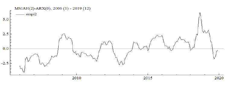
Figure B2
Probabilities of Regime 1 (Low-Pressure Regime)

 

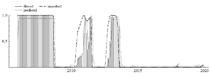
Figure B3
Probabilities of Regime 2 (High-Pressure Regime)

 

Source: Authors’ calculations

Appendix C

Table C1
Estimation Results (Robustness Check)

Regime 1 (n: 55.4, Prob.: 0.259, Duration: 18.18, Std. Error: 0.616)
Variable	Coefficient	Standard Error	t-value
α	-1.566***	0.210	-7.433
yt	0.820***	0.210	3.894
πt	1.154***	0.347	3.326
crdtt	-0.569***	0.121	-4.699
stdt	0.293***	0.109	2.693
vixt	-0.217*	0.126	-1.725
∇it	0.301	0.272	1.103
Regime 2 (n:112.6, Prob: 0.740, Duration: 51.86 Std. Error: 0.556)
Variable	Coefficient	Standard Error	t-value
α	0.874***	0.093	9.386
yt	-0.532***	0.079	-6.675
πt	0.766***	0.100	7.606
crdtt	1.336***	0.105	12.641
stdt	-1.175***	0.127	-9.243
vixt	0.053	0.082	0.647
∇it	-0.247*	0.141	-1.744

LR Linearity Test: 194.403	Chi (8) = (0.000)***	Chi (10) = (0.000)***
	Log-likelihood	AIC
Nonlinear model	-162.695	2.151
Linear model	-259.896	3.189

Note. ***, **, and * indicate significance at 1%, 5%, and 10%, respectively.
Source: Authors’ calculations