Organizations and Markets in Emerging Economies ISSN 2029-4581 eISSN 2345-0037
2023, vol. 14, no. 2(28), pp. 436–457 DOI: https://doi.org/10.15388/omee.2023.14.99
Heuristic Rules for the Dynamic Pricing Problem
Oleg Melnikov
National Technical University “Kharkiv Polytechnic Institute”, Ukraine
https://orcid.org/0000-0002-2409-4983
Oleg.Melnikov@khpi.edu.ua
Abstract. This paper is devoted to the development of heuristics for the dynamic pricing problem. A discrete time model of dynamic pricing on the fixed time horizon is proposed. It is applicable to products that satisfy two properties: 1) product value expires at a certain predetermined date, and 2) consumers demand at most a single unit of the product. This type of demand structure allows deriving a simple system of recursive equations for optimal prices using dynamic programming techniques. Optimal pricing policy is expressed as a function of time to expiration and inventory levels of unsold products. An analytical solution to this problem was obtained for special cases, while for the general case, a numerical algorithm has been developed. Qualitative characteristics of the optimal pricing policy are established, and their implications for dynamics of inventories and prices are discussed. Based on these observations, a simple heuristic rule for dynamic price adjustments is proposed. Performance of this heuristic is evaluated against the optimal dynamic and fixed-price policies using Monte-Carlo experiments. Results demonstrate high efficiency of the proposed heuristic strategy and its even simpler derivatives. Heuristics’ adaptability and ease of implementation should make it suitable and attractive for small and medium businesses.
Keywords: dynamic pricing, revenue management, price discrimination, inventory, backward induction, dynamic programming, heuristics
Received: 19/11/2022. Accepted: 27/4/2023
Copyright © 2023 Oleg Melnikov. Published by Vilnius University Press. This is an Open Access article distributed under the terms of the Creative Commons Attribution Licence, which permits unrestricted use, distribution, and reproduction in any medium, provided the original author and source are credited.
1. Introduction
Dynamic pricing is commonly defined as a strategy of flexibly changing sales prices depending on market conditions (Deksnyte & Lydeka, 2012). This definition is somewhat imprecise as the ability of prices to adapt to changing environment is the main element that ensures proper functioning of the market mechanism. However, the frequency of price adjustments is not always high. Among factors that slow down the pace of price changes entrepreneurs often cite:
• lack of operational information;
• time required to realize the changes that have taken place;
• high costs associated with price changes (Elmaghraby & Keskinocak, 2003).
Some prominent economists (in particular, of the Keynesian and Neo-Keynesian schools) even consider excessively static “sticky” prices to be one of the main factors of periodic economic crises (Barro & Tenreyro, 2006) and failures of macroeconomic regulatory policies (Wang & Werning, 2022).
Development of electronic commerce provides companies with more opportunities for prompt price adjustments. This is facilitated by:
• availability of large volumes of data on the structure of demand in real time (data on site visits, sales conversion, etc.);
• low costs for changing sales prices;
• possibility of integrating complex price adjustment algorithms directly into the general software environment of the online store.
These considerations have intensified interest in dynamic pricing algorithms for sales management. These algorithms automatically apply a computerized rule to set prices based on various inputs. These inputs commonly include demand and supply conditions, competitors’ prices, customer demographics and preferences, time of day, day of the week, and time of year (MacKay & Weinstein, 2022). Pricing algorithms allow firms, particularly e-commerce firms, to update and optimize their pricing quickly and continuously. Dynamic pricing is a form of price discrimination where different buyers pay different prices for the same product.
Dynamic pricing methods have gained particular popularity in those industries where it is difficult to change the supply of goods in the short term. Examples of such situations can be the sale of tickets for flights, trains, concerts, or sports events; hotel reservations; road tolls; gas and electricity supply services, etc. Dynamic pricing strategies have become especially popular when selling airplane seats, where the price of the ticket for the same flight can vary by an order of magnitude depending on the season, day of the week, time before departure, booking conditions and other factors (Malighetti et al., 2009; Wittman & Belobaba, 2019).
Figure 1 represents an example of this pricing pattern which shows ticket prices for one-way Wizzair Vilnius-Milan flight sampled at different times for various departure dates. Even in this small sample, prices range almost by a factor of three (from €50 to €145). It is also evident that there is no set pattern for the change in prices: although in most cases prices increase as departure date nears, for departures on 9/26 and 10/10, seat prices had declined.
Other industries where dynamic pricing is widespread include hospitality (Gibbs et al., 2018), entertainment (Bouchet et al., 2016), retail (Hendel & Nevo, 2013), public transportation (Branda et al., 2020), etc.
Figure 1
Prices for Wizzair Vilnius-Milan Malpensa Flight Seats Sampled at Different Dates Prior to Departure
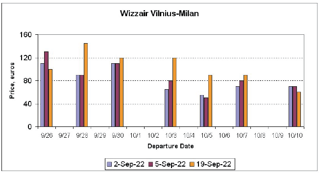
Note. Retrieved from https://wizzair.com on specified dates.
The success of such practices promotes their spread to other areas of the economy as well. The development of automated trading systems also facilitates implementation of dynamic pricing mechanisms. The advent of artificial intelligence and big data analytics allows for increasingly more complicated pricing rules.
However, this increasing sophistication should not deter small and medium businesses from employing dynamic pricing mechanisms. Many pricing regularities that arise in dynamic pricing algorithms are simple and intuitive. The objective of this paper is to explore such regularities and to develop simple, practical and easy to implement dynamic pricing heuristics on this basis. This fills a gap in the literature concerned with practical adoption of dynamic pricing techniques, which may be especially relevant to entrepreneurs in the emerging economies where limited resources often make using expensive dedicated software impractical.
The rest of the paper is organized as follows. Section 2 reviews key literature on dynamic pricing. Section 3 presents a simple model of dynamic pricing based on inventory fluctuations and establishes important properties of the optimal pricing policy. Section 4 analyzes common patterns of price and inventory behavior that arise in the above model and suggests several heuristic pricing rules on this basis. Section 5 estimates benefits from adopting dynamic pricing and evaluates performance of suggested heuristics vs. the optimal pricing policy via analytical calculations and numerical Monte Carlo experiments. Results show that proposed heuristic rules sacrifice very little in terms of performance while being much easier to implement. The last section concludes and discusses some possible venues for further research.
2. Literature Overview and Research Objectives
Probably, the idea of changing prices dynamically to maximize revenue from product sales was first proposed and rigorously studied by Kincaid and Darling (1963), whose work did not become widely known until much later.
Lazear (1986) considered the problem of selling an indivisible product to homogeneous consumers with an unknown demand function, which the seller can gradually learn by changing prices. He showed that the optimal policy for the seller is to slowly lower prices over time, effectively employing a practice known as “clearance” in retailing and as “price skimming” in general marketing. Early empirical papers investigated dynamic pricing patterns common in retail industry and tried to explain them using various hypotheses, such as fashion hypothesis (Lazear, 1986; Pashigian, 1988; Pashigian & Bowen, 1991), peak-load pricing (Chao, 1983), and the thick-market hypothesis (Warner & Barsky, 1995).
Perhaps the most influential study on this topic is the work of Gallego and van Ryzin (1994). They modeled demand as a time-invariant Poisson process with an intensity that depends on the selling price. Calculus of variations is employed to derive differential equations for the optimal control policy. The authors obtain an analytical solution for the exponential demand function and establish some properties of the optimal pricing policy for a more general case.
There are many modifications and extensions of the Gallego-van Ryzin model. Gallego and van Ryzin (1997) extended their model to the case of multiple products with possibly interconnected demand. Bitran and Mondschein (1997) and Zhao and Zheng (2000) model demand as a non-homogenous Poisson process and allow the elasticity of demand to change over time. Smith and Achabal (1998) and Mantrala and Rao (2001) consider initial inventory decisions in conjunction with markdown pricing decisions.
All these models call for the continuous updating of prices over time, which is rarely practical. Gallego and van Ryzin (1994) also considered a scenario where the price must be chosen from a discrete set of allowable prices. Under this assumption, price changes become less frequent. Feng and Gallego (1995) proposed a model that allows for a single possible price change during the planning horizon and optimizes the timing of such change. Feng and Xiao (2000) allow for several price changes during the season. Aguirregabiria (1999) accounts for the “menu costs” of changing prices, which produces a similar effect of lowering the frequency of price adjustments.
A detailed review of these studies can be found in Elmaghraby and Keskinocak (2003).
All studies mentioned above treat consumer behavior as myopic. A different line of research studies the implications of strategic, forward-looking behavior on consumers’ side. This topic is largely motivated by the classic work of Nobel Laureate Ronald Coase (1972), which questioned the effectiveness of the skimming policy. According to Coase,
rational consumers will anticipate future price reductions and thus postpone their decision to buy the product, which in turn will force the seller to immediately reduce prices, even in a monopoly case. The role of expectations and forward-looking consumer behavior for sales management was analyzed by Su (2007), Melnikov (2013), Levin et al. (2009), among others.
Talluri and Van Ryzin (2004) employed discrete choice models to study the situation when consumer’s purchase decision depends not only on price but also on other factors such as proximity of the expiration date. This may be particularly relevant to the airline industry, where it is commonly believed that the overall market can be segmented into (at least) two classes: early-booking leisure travelers and late-booking business travelers. Williams (2022) findings seem to confirm this conjecture based on a large dataset on US airlines fares.
A large body of research is devoted to the use of machine learning algorithms to estimate the intensity of consumer flow and the impact of prices on purchase probabilities, from classical as well as from Bayesian perspective. Den Boer (2015) provides a comprehensive survey of related literature. Recent important additions to this line of research include Avramidis (2020) and Wang et al. (2021).
There are many empirical studies that investigate dynamic pricing practices in various industries, such as airlines (Malighetti et al., 2009; Wittman & Belobaba, 2019; Williams, 2022), hotels (Gibbs et al., 2018), retail (Hendel & Nevo, 2013), public transportation (Branda et al., 2020), food delivery (MacKay et al., 2022) and others.
However, despite a large body of research, many aspects of dynamic pricing remain controversial. They include, among others:
• assessment of the profitability of this strategy versus more common fixed prices;
• welfare implications of dynamic pricing;
• applicability of dynamic pricing to particular industries;
• common pricing patterns that emerge from employing dynamic pricing;
• development of simple heuristic pricing rules that would facilitate adoption of dynamic pricing by small and medium businesses.
This paper aims to develop a model of dynamic adaptive pricing for the sale of products whose value expires with time, which is easy to estimate and to implement practically. In contrast to the Gallego-van Ryzin model, we use a discrete time setting and model demand as a composite process which is a superposition of consumer arrivals and price-dependent conversion rates. To simplify the model further, we consider the case of discrete demand, when each individual consumer is interested in acquiring at most a single unit of a product. A typical example of such demand structure is the above mentioned sale of airline tickets, when it is necessary to sell a fixed number of seats in the cabin before the departure of the flight. Similar situations arise when selling hotel rooms, tickets to concerts and sporting events, perishable goods, and so on.
This type of demand structure leads to a computationally simple model which can be solved analytically in some special cases. For the general case, it is possible to establish qualitative properties of the optimal policy. This allows devising simple heuristics which are easy to implement without extensive software support.
3. The Model
Consider a simple single-agent, homogeneous products model. The seller has X units of a homogeneous product to sell over a finite time interval t = 1, ..., T. All costs related to procurement of these units are sunk, so the seller’s objective is to maximize their expected revenue. Product value expires at time T. This assumption is applicable to different industries, including travel (airplane seats, hotel rooms), retailing (perishable products, fashion apparel, seasonal goods), and entertainment (concerts, sport events).
Customers arrive continuously according to a constant intensity deterministic flow. We normalize the number of periods so that customer arrival rate equals exactly one customer per time period. Each customer demands a single unit of the seller’s product. Consumer arriving at time t is willing to pay at most rt for a unit of product, a value which will be referred to below as a consumer’s reservation price (Steedman, 1987). Further assume that rt are independent identically distributed random variables drawn from the distribution given by cumulative distribution function F(r) with a finite support 0 ≤ rt ≤ v.
A consumer arriving at time t buys one unit of a good if pt ≤ rt , where pt is the price charged by the seller. Thus, the probability of sale in period t equals the value of the complementary distribution function G(pt) = 1 – F(pt). Otherwise, the consumer buys nothing, and the process restarts at the next period with the same inventory level. Given these assumptions, the expected demand at time t would be equal to G(pt), so G(pt) can be interpreted as the usual demand function.
Let xt denote remaining stock at the beginning of period t and assume for simplicity zero storage costs.
The seller’s problem is to maximize the following objective function over a sequence of prices pt :
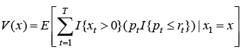 (1)
(1)
subject to
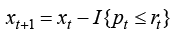 (2)
(2)
where E[∙|∙] is the conditional expectation operator, and I{∙} is the indicator function.
It is easier to derive the optimal pricing policy and establish its properties by considering first the special case when x = 1, that is, when the seller has a single indivisible unit of a product to sell. This might be of interest by itself for such instances as selling real estate, art objects, and other unique products.
3.1 Single Unit Case
The problem is easy to solve by backward induction (Stokey & Lucas, 1989; Judd, 1998). Denote by Vt the maximum expected income of the seller in period t, if the product has not yet been sold by that time. According to the boundary condition of the problem, Vt+1. For the last time period, the optimal price and expected seller’s gain can be found from
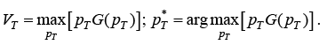 (3)
(3)
Knowing the seller’s optimal policy in the last period, we can formulate their optimization task in the penultimate period. When setting the price, two results are possible:
1) the product will be sold, and the seller will receive revenue of pT–1. The probability of this result is equal to G(pT–1);
2) the product will not be sold with complementary probability 1 – G(pT–1). Then the seller will find himself/herself in the conditions of problem (3), for which the optimal solution was already derived.
Thus, expected seller’s gain at period t-1 is given by
 (4)
(4)
Continuing in this fashion, we will get a solution to the problem for an arbitrary time period. It will be determined as a solution to the equation
 (5)
(5)
Proposition 1 establishes some properties of the optimal pricing policy.
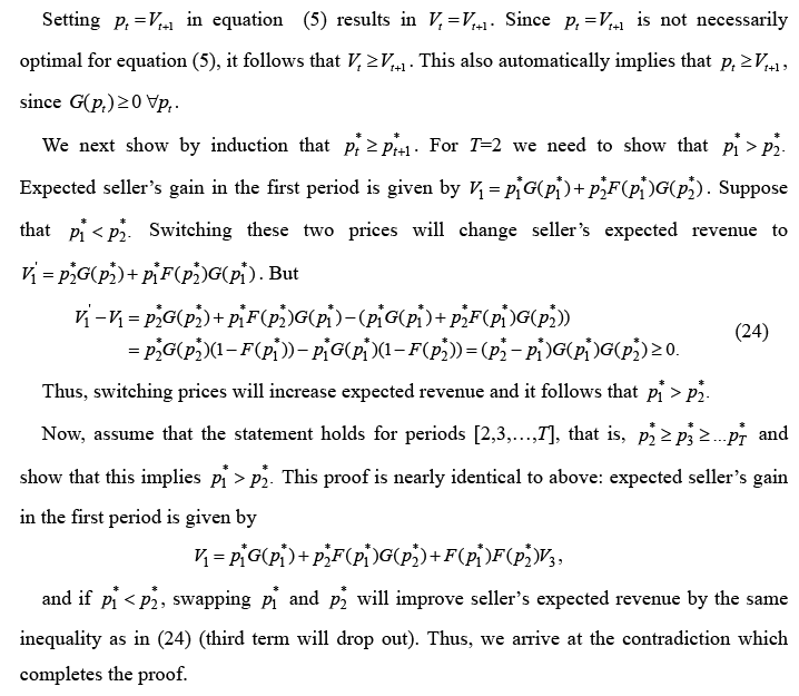
Proposition 1. Expected seller’s gain and optimal prices are both non-increasing functions of time:
Proof of this proposition is given in Appendix A.
A pattern of gradually declining prices is known as the skimming strategy in marketing. Proposition 1 establishes that price skimming is indeed optimal for sales of unique products.
For a numerical example, consider the special case with uniform U(0,1) distribution of reservation prices. Then F(p) = p; G(p) = 1 – p, and equation (5) simplifies to
 (6)
(6)
First-order optimality condition for problem (6) is given by
 (7)
(7)
from which it follows that
 (8)
(8)
Figure 2 shows the graph of the optimal price as a function of time. It also plots numerically computed optimal prices for the case where reservation prices are normally distributed. Parameters of the normal distribution are chosen so that the bulk of the distribution is concentrated on the unit interval, and results are directly comparable with the uniform distribution case. It is easy to see that without time pressure optimal prices flatten out, converging to the upper bound of the distribution of consumer prices. However, if the product remains unsold as the expiration time approaches, the seller is likely to offer substantial price discounts.
Figure 2
Optimal Prices for a Single Product as a Function of Time
3.2 Multiple Units Case
Now let us return to the general case with multiple countable units of a homogeneous product to sell.
Clearly, it is easier to sell a smaller number of products within any given time frame. Thus, the price of products in each period should depend not only on time, but also on the stock of unsold products xt . Accordingly, we will look for the optimal prices in the form of a feedback loop, with inventories xt as a state variable. To this end, define V xt and p xt to be the expected revenue and the price as of time t, correspondingly, when the current inventory level equals x.
We maintain the assumption that a single period demand cannot exceed one unit. Thus, at any point in time there are two possible outcomes of the seller’s interaction with a potential buyer:
1) the product is not sold at the current price. Then in the current period t, the seller receives no income and moves on to the next period with unchanged stocks, xt+1 = x;
2) the product is successfully sold. Then in the current period, the seller receives income p xt and proceeds to the next period with the stock level xt+1 = x – 1.
Combining these two possibilities, we arrive at the following Bellman equation for dynamics of the value function V xt :
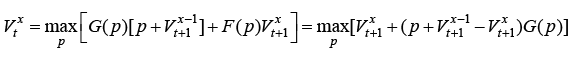 (9)
(9)
subject to the boundary conditions
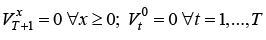 . (10)
Optimal state-dependent prices p xt are then determined as a solution to the optimization problem (9). First order optimality conditions for this problem are
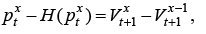 (11)
(11)
where H(p xt ) is an inverse value of the hazard rate,
 (12)
(12)
and f(p) = dF(p) / dp is a probability density function.
Plugging (11) into (9) gives
 (13)
(13)
Numerically, the above problem can be solved by backward induction. Combining optimality conditions (11) with boundary conditions (10) yields
 (14)
(14)
Thus, the last period optimal price is independent of x. Equation (14) can be rearranged as
 (15)
(15)
Given that G(p) can be interpreted as a demand function, the last equation just restates a familiar rule that the revenue-maximizing price corresponds to the point where demand curve is unit-elastic.
Plugging p xT into equation (13) we obtain V xt , solve for p xt–1 using optimality conditions (11) and so on.
Expression on the left-hand side of equation (11) is known as the virtual valuation in the auction literature (Myerson, 1981). A probability distribution function F(p) is called regular if its virtual valuation function is weakly increasing. A sufficient condition for regularity is monotone hazard rate (which in turn implies that its inverse H(p) will be weakly decreasing). This condition is satisfied for the majority of commonly used distributions.
Properties of the optimal pricing policy and seller’s expected revenue are established by the following:
Proposition 2.
2.1) Expected seller’s revenue V xt is a weakly decreasing function of t.
2.2) Expected seller’s revenue V xt is a weakly increasing function of x.
2.3) Optimal pricing policy p xt is a weakly decreasing function of t.
2.4) If the distribution of consumer reservation values has monotone hazard rate, then optimal pricing policy p xt is a weakly decreasing function of x.
Proof of these propositions is given in Appendix B.
As a numerical example, let’s continue the case of uniform distribution of reservation prices considered above. For x=1, the sequence of optimal prices p 1t is already found and given by equation (8). From equation (14) it follows that  N. Then, applying iteratively formulae (13) and (11) for t = T–1, T –2, ... and or x = 2, 3, ..., we arrive at the following sequence:
 (16)
(16)
Figure 3 shows these price sequences for x=5 and T=30.
Figure 3
Optimal Prices as a Function of Time and Remaining Stock Levels, rt~U(0,1)
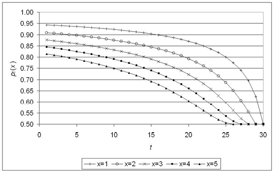
A combination of pricing policy properties established by Proposition 2.2 makes the observed behavior of prices much more complicated than in the single product case. Observed price pt belongs to the set 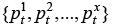 , but true value of xt is known to the seller but not to the buyer. With stable stock levels, prices will be gradually lowered over time. However, when sale happens, inventory levels drop, and the optimal price jumps from p xt to
  , which must be higher than p xt by Proposition 2.2. This may cause observed prices to rise sharply. As the timing of successful sales is random, so is the observed price path.
The mechanism of this process is illustrated in Figure 4, where price fluctuations (black line) are superimposed on possible inventory movements (blue line) obtained as a result of computer simulation (this and subsequent figures assume standard uniform distribution of consumers’ reservation prices unless explicitly stated otherwise).
Figure 4
Price Adjustment Mechanism
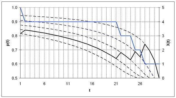
Figure 5
Some Simulated Price Paths
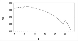
Figure 5 shows results of several computer simulations that illustrate possible price dynamics that may arise in the above model. As evident from these graphs, prices may decline over time just as easily as they can rise up.
4. Implementation and Simple Pricing Heuristics
The assumptions made about the structure of demand for seller’s products impose certain restrictions on the possible inventory evolution patterns. As one-period demand is at most one unit, total sales cannot exceed the number of periods. However, realistic sales targets should be much lower. Propositions 2.3 and 2.4 imply that the minimum price the seller would ever charge is the last period price, given by the solution of equation (14). Let us denote this price by pmin. Then in the absence of inventory constraints, the expected sales for T periods would be equal to Xe(T) = TG(pmin). For example, for rt ~U[0,1], pmin =1/2 and Xe(T) = T/2. Hence, higher values of initial inventories are unlikely to sell out.
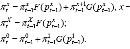
Equations 11–13 jointly create a Markov chain for the evolution of inventories Xt during the sales period. It has a structure identical to the pure death processes common in queuing theory (Ross, 1992). Exact distribution of inventory levels at any given time 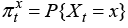 can be obtained from the following system of recursive equations:
 (17)
(17)
The initial probability distribution under X0 = X is given by 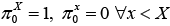 .
.
In turn, the distribution of inventories jointly with the set of state-dependent prices p xt defines the distribution of observed product prices, sales, inventories, seller’s revenues and any other numerical characteristics of stochastic processes Xt , pt and their derivatives for each time period. For instance, expected inventory levels as a function of time can be obtained as
 (18)
(18)
Figure 6 shows how expected inventory levels change over time depending on initial stocks.
The above graph allows making some observations on the qualitative properties of the optimal pricing policy. Expected inventory paths are close to linear. When initial stocks are comparatively low (below Xe(T)), prices are set so as to sell out inventories by the end of the period. If initial stocks are high, prices are set to sell out as much as possible, at the level close to pmin. In both scenarios expected sales intensity is approximately constant.
Figure 6
Expected Inventory Levels as a Function of Time for Various Starting Values
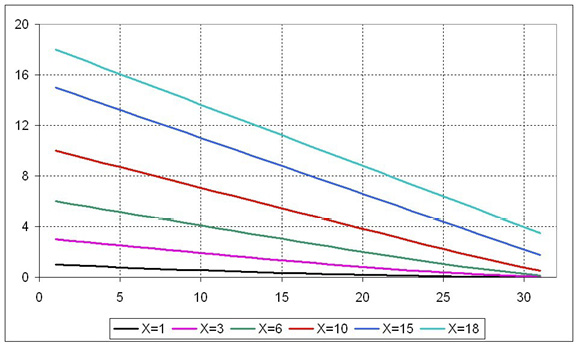
Note. X0=X, T=30.
These observations suggest the following simple heuristic rule for dynamic pricing. To achieve sell-out of x inventory units in t periods of time, the expected per-period sales should equal x/t. Define the sell-out price pso(x, t) as a solution to the equation G(p) = x/t or
 (19)
(19)
where F–1(•) is an inverse of the cumulative distribution function and assuming x≤t. Then set the current price pt according to the rule
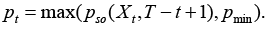 (20)
(20)
This heuristic rule is much simpler to implement than the full model (11)-(13) as it only requires solving a single equation (20), which often allows for an analytical solution; for example, in the uniform case 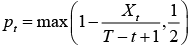 . It also has a simple and intuitive interpretation. Each period current inventories are compared against their target level, which is assumed to evolve linearly over time so that inventories would sold out by the end of their expiration value. If sales proceed faster than planned, product prices rise. When sales process slows down compared to the target, prices fall. If it becomes apparent that inventories cannot be sold by the end of the selling period, prices are set at the minimum acceptable level, which maximizes per-period revenue rate.
The proposed heuristic rule still requires changing prices every period. In many cases, this is not practical. It is easy to make up some derivative heuristic rules based on equation (20) which would limit the frequency of price adjustments. These rules may impose changing prices only at certain predetermined time intervals (e.g., on a weekly basis) or when a certain event happens (e.g., when current sales deviate from their target level by a certain threshold).
Performance of the proposed heuristic (20) and of some derivative rules will be evaluated in the next section.
5. Benchmarking
To assess efficiency of the dynamic pricing strategy and proposed heuristics, it is worthwhile discussing alternative pricing rules. The obvious yardstick for comparing performance is a fixed price policy. However, finding the optimal fixed price for the above problem is not trivial.
If prices were to remain constant at pt = p during sales period, the probability of a sale in any given period would also be constant equaling to λ = G(p). Evolution of sales can be modeled as a Markov chain, which is reduced to the following system of recursive equations:
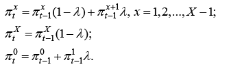 (21)
(21)
Then seller’s expected revenue as of time t can be found as
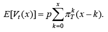 (22)
(22)
Alternatively, one can view a successful sale as a success in series of independent trials, each trial being a single interaction between the seller and a buyer. Were it not for the limited stocks, the distribution of sales on [t, T] would be binomial with T – t + 1 trials and success probability λ. Taking inventory considerations into account, sales over [t, T] can be viewed as a random variable St = min{Z, xt}, where Z ~ B(T – t + 1, λ), and expected revenue is then
E[Vt(x)] = pE[St]. (23)
Optimal fixed price PFP can be found by maximizing objective functions (22) or (23) over p. Interestingly, even in the uniform case used in examples above, this would require employing numerical optimization routines.
One exemption is the case of selling a single product. At the fixed price p, the probability that a product will not be sold during T periods of time equals (F(p))T. Hence, the probability of a successful sale equals 1 – (F(p))T, and the seller’s expected revenue is given by p[1 – (F(p))T]. The optimal fixed price can be found by maximizing the above expression over p. For the uniform case rt~U(0,1), it is straightforward to show that the optimal fixed price equals (1+T)1/T. Expected revenue can be obtained by plugging this formula into formula (22).
Evaluating performance of different pricing strategies is not straightforward, either. In general, payoff of a particular strategy depends on factors such as:
• starting inventory level;
• length of the selling period;
• shape of the distribution of consumers’ reservation prices;
• point in time when evaluation is performed, etc.
It is not possible to account for all these variables in a single graph, so at least some of them should be held constant for a meaningful interpretation.
Figure 7
Comparison of the Seller’s Expected Revenue under Fixed and Flexible Prices
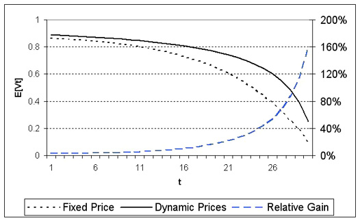
Note. rt~U(0,1), X = 1, T = 30.
Figure 7 illustrates the main payoff from using dynamic pricing. It compares expected seller’s revenues under the optimal fixed price policy pFP (dotted line) and under dynamic price adjustment (solid line) for the single unit case if that unit remains unsold at the current point in time. Relative efficiency of employing the second strategy is also shown.
As can be seen from the graph, sticking to a predetermined price becomes progressively inefficient as time goes by and chances of a successful sale diminish. For the above scenario, the gain from employing dynamic pricing approaches 159% in relative terms towards the end of the selling period. However, chances are that the product will be sold long before that under both pricing strategies, so the above graph illustrates the worst-case scenario for the seller.
A more objective way to compare performance of different strategies is to compute their ex-ante expected payoff. Figure 8 compares expected revenues from selling a single unit of a product for T periods as a function of T for the following strategies:
• optimal dynamic pricing strategy (optimal);
• fixed price set at the beginning of the selling period at the level of (20) (sellout);
• optimal fixed price pFP (optimal fixed price);
• dynamic pricing in accordance with the heuristic rule (20) (heuristic);
• heuristic rule (20) with price changes allowed every 10 periods (limited adjustments).
Figure 8
Comparison of the Seller’s Ex-ante Expected Revenues
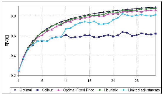
Note. Revenues under different strategies as a function of T(rt~U(0,1), X = 1).
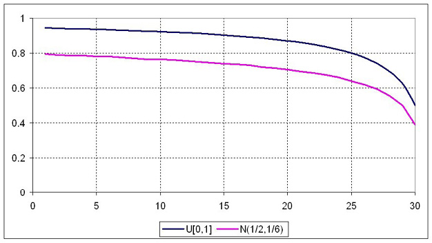
Figure 9
Performance Indices of Different Strategies
a) 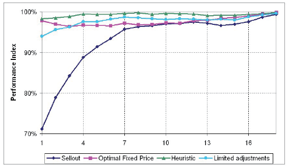
b) 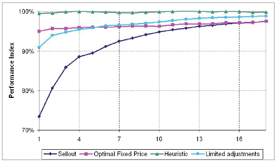
Note. Performance as a function of starting inventory levels: (a) rt~U(0,1), T = 30); (b) rt~N(1/2, 1/6), T = 30).
Expected values for the optimal strategy were computed using formula (8), while for the other strategies they were averaged out after running 1000 computer simulations.
Figures 9a and 9b provide similar calculations while holding fixed the number of periods (T), while changing the starting inventory levels (X). For a more visual comparison, a performance index for each strategy was calculated as a ratio of its expected payoff to the payoff of the optimal strategy. Optimal strategy for the normal distribution was computed numerically.
Figure 10 shows expected closing stocks of unsold units from the same set of experiments as in Figure 9a. It shows that the proposed heuristic pricing rule is somewhat more aggressive than optimal as it results in the higher number of units sold. On the other hand, optimal fixed price policy results in underselling stocks relative to the optimal strategy.
Figure 10
Expected Closing Stocks for Different Strategies
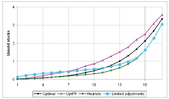
Note. Closing stocks as a function of the starting inventory levels (rt~U(0,1), T = 30).
The above calculations show that the proposed heuristic rule performs very well overall, within 2% error bounds from the optimal strategy even in the worst case scenario. A simplified heuristic rule with a limited price adjustment frequency also performs reasonably except for the very low initial inventory levels. As these strategies are much easier to implement in comparison to the full dynamic optimization model, their adoption may benefit small and medium businesses.
6. Conclusions and Directions for Further Research
The model developed above allows determining optimal prices as a function of inventory levels and time remaining to the expiration of the product value. Calculations and computer simulations show that employing dynamic pricing can bring a substantial payoff in comparison to the more common static prices strategy. The established properties of the optimal pricing mechanism allow developing fairly simple and intuitive heuristic rules for dynamic price adjustments.
There are several directions where this line of research can be extended. From theoretical perspective, optimal conditions for the pricing policy are very similar to those that arise in the auction literature. This is especially apparent for the single unit case, where the pricing pattern is reminiscent of the Dutch auction (Klemperer, 2004). The resemblance is likely due to the fact that both dynamic pricing and auctions can be thought of as price discovery mechanisms striving to sell the product to the highest bidder(s). Exploring this avenue may bring up some useful theoretical generalizations.
From empirical perspective, it is interesting to explore to which extent the above model may account for typical pricing patterns and the degree of price dispersion present in particular markets.
Practical implementation of the above model requires estimates of the intensity of consumer flow and price-dependent conversion rates, which may not be readily available. There is a growing body of research on using machine learning algorithms and analytical processing of the sales data for estimating a demand function. However, most of these algorithms require extensive price experimentation and processing of the large amounts of data. Both of these features may make employing such algorithms too costly for small and medium businesses, which might prefer using simple and robust heuristics instead. The suggested pricing heuristic can be thought of as a simple feedback controller based on the difference between the actual and desired sales dynamics. Such schemes are known to be fairly robust to model misspecifications, although evaluating performance of the suggested pricing rule under incomplete demand knowledge lies beyond the scope of this paper.
Another interesting expansion of the model would be treating the above problem as a repeating process and endogenizing the sales horizon. This would bridge pricing decisions with the classical inventory management problems such as determining the optimal order size, replenishment frequency and so on.
Exploring these and other issues related to dynamic pricing may be of substantial theoretical and practical interest.
References
Aguirregabiria, V. (1999). The Dynamics of Markups and Inventories in Retailing Firms. The Review of Economic Studies, 66(2), 275–308.
Avramidis, A. N. (2020). A Pricing Problem with Unknown Arrival Rate and Price Sensitivity. Mathematical Methods of Operations Research, 92, 77–106.
Barro, R. J., & Tenreyro, S. (2006). Closed and Open Economy Models of Business Cycles with Marked Up and Sticky Prices. The Economic Journal, 116(511), 434–456.
Bitran, G., R., & Mondschein, S. V. (1997). Periodic Pricing of Seasonal Products in Retailing. Management Science, 43(1), 64–79.
Bouchet, A., Troilo, M., & Walkup, B.R. (2016). Dynamic Pricing Usage in Sports for Revenue Management. Managerial Finance, 42(9), 913–921. https://doi.org/10.1108/MF-01-2016-0017
Branda, F., Marozzo, F., & Talia, D. (2020). Ticket Sales Prediction and Dynamic Pricing Strategies in Public Transport. Big Data and Cognitive Computing, 4(4), 36, 1–17. doi:10.3390/bdcc4040036
Chao, H.-P. (1983). Peak Load Pricing and Capacity Planning with Demand and Supply Uncertainty. Bell Journal of Economics, 14(1), 170–190.
Coase, R. H. (1972). Durability and Monopoly. Journal of Law & Economics, 15(1), 143-149.
Dean, J. (1976) Pricing Policies for New Products. Harvard Business Review, 54(6), 141–153.
Deksnyte, I., & Lydeka, Z. (2012). Dynamic Pricing and Its Forming Factors. International Journal of Business and Social Science, 3(23), 213–220.
Den Boer, A. V. (2015). Dynamic pricing and learning: Historical origins, current research, and new directions. Surveys in Operations Research and Management Science, 20(1), 1–18.
Elmaghraby, W., & Keskinocak, P. (2003). Dynamic Pricing in the Presence of Inventory Considerations: Research Overview, Current Practices, and Future Directions. Management Science, 49(10), 1287–1309.
Feng, Y., & Gallego, G. (1995). Optimal Starting Times for End-of-Season Sales and Optimal Stopping Times for Promotional Fares. Management Science, 41(8), 1371–1391.
Feng, Y., & Xiao, B.(2000). Optimal Policies of Yield Management with Multiple Predetermined Prices. Operation Research, 48(2), 332–343. https://doi.org/10.1287/opre.48.2.332.13373
Gallego, G., & van Ryzin, G. (1994). Optimal Dynamic Pricing of Inventories with Stochastic Demand over Finite Horizons. Management Science, 40(8), 999–1020.
Gallego, G., & van Ryzin, G. (1997). A Multiple Product Dynamic Pricing Problem with Applications to Network Yield Management. Operation Research, 45(1), 24–41.
Gibbs, C., Guttentag, D., Gretzel, U., Yao, L., & Morton, J. (2018). Use of Dynamic Pricing Strategies by Airbnb Hosts. International Journal of Contemporary Hospitality Management, 30(1), 2-20. https://doi.org/10.1108/IJCHM-09-2016-0540
Hendel, I., & Nevo, A. (2013). Intertemporal Price Discrimination in Storable Goods Markets. American Economic Review, 103(7), 2722–2751. DOI: 10.1257/aer.103.7.2722
Judd, K. L. (1998). Numerical Methods in Economics. Cambridge & London: The MIT Press.
Kannan, P. K., & Kopalle, P. K. (2001). Dynamic Pricing on the Internet: Importance and Implications for Consumer Behavior. International Journal of Electronic Commerce, 5(3), 63–83.
Kincaid, W. M., & Darling, D. (1963). An Inventory Pricing Problem. Journal of Mathematical Analysis and Applications, 7, 183–208.
Klemperer, P. (2004). Auctions: Theory and Practice. Princeton, N. J.: Princeton University Press.
Lazear, D. P. (1986). Retail Pricing and Clearance Sales. American Economics Review, 76(1), 14-32.
Levin, Y., McGill, J, & Nediak, M. (2009). Dynamic Pricing in the Presence of Strategic Consumers and Oligopolistic Competition. Management Science, 55(1), 32–46.
MacKay, A., Svartback, D., & Ekholm, A. G. (2022). Dynamic Pricing and Demand Volatility: Evidence from Restaurant Food Delivery (Harvard Business School Working Paper 23-007). Available at SSRN 4164271
MacKay, A. J., & Weinstein, S. N. (2022). Dynamic Pricing Algorithms, Consumer Harm, and Regulatory Response (Harvard Business School Working Paper 22-050). Available at: http://dx.doi.org/10.2139/ssrn.3979147. 55pp.
Malighetti, P., Paleari, S., & Redondi, R. (2009). Pricing Strategies of Low-cost Airlines: The Ryanair Case Study. Journal of Air Transport, 15(4), 195–203.
Mantrala, M. K., & Rao, S. (2001). A Decision-Support System that Helps Retailers Decide Order Quantities and Markdowns for Fashion Goods. Interfaces, 31(3), S146–S165.
Melnikov, O. (2013). Demand for Differentiated Durable Products: The Case of the U.S. Computer Printer Market. Economic Inquiry, 51(2), 1277-1298.
Myerson, R. B. (1981). Optimal Auction Design. Mathematics of Operations Research 6(1), 58–73. doi:10.1287/moor.6.1.58
Pashigian, B. P. (1988). Demand Uncertainty and Sales: A Study of Fashion and Markdown Pricing. American Economic Review, 78(5), 936–953.
Pashigan, B. P., & Bowen, B. (1991). Why Are Products Sold on Sale?: Explanations of Pricing Regularities. The Quarterly Journal of Economics, 106(4), 1014-1038.
Ross, S. M. (1992). Applied Probability Models with Optimization Applications. New York: Dover Publications, Inc.
Smith, S., & Achabal, D. (1998). Clearance Pricing and Inventory Policies for Retail Chains. Management Science, 44(3), 285–300. https://doi.org/10.1287/mnsc.44.3.285
Steedman, I. (1987). Reservation Price and Reservation Demand. In The New Palgrave Dictionary of Economics (Vol 4, pp. 158–59).
Stokey, N. L., & Lucas, R. E. (1989). Recursive Methods in Economic Dynamics. Cambridge & London: Harvard University Press.
Su, X. (2007). Intertemporal Pricing with Strategic Customer Behavior. Management Science, 53(5), 726–741. https://doi.org/10.1287/mnsc.1060.0667
Talluri, K., & Van Ryzin, G. (2004). Revenue Management Under a General Discrete Choice Model of Consumer Behavior. Management Science, 50(1), 15–33.
Wang, O., & Werning, I. (2022). Dynamic Oligopoly and Price Stickiness. American Economic Review, 112(8), 2815-2849. DOI: 10.1257/aer.20201739
Wang, R., Gan, X., Li, Q., & Yan, X. (2021). Solving a Joint Pricing and Inventory Control Problem for Perishables via Deep Reinforcement Learning. Complexity, Article ID 6643131.
Warner, E. J., & Barsky, R. B. (1995). The Timing and Magnitude of Retail Store Markdowns: Evidence from Weekends and Holidays. Quarterly Journal of Economics, 110(2), 321–352.
Williams, K. R. (2022). The Welfare Effects of Dynamic Pricing: Evidence from Airline Markets. Econometrica, 90(2), 831–858. doi:10.3982/ecta16180
Wittman, M. D., & Belobaba, P. P. (2019). Dynamic Pricing Mechanisms for the Airline Industry: A Definitional Framework. Journal of Revenue and Pricing Management, 18, 100-106. https://hdl.handle.net/1721.1/128436
Zhao, W., & Zheng, Y. (2000). Optimal Dynamic Pricing for Perishable Assets with Nonhomogeneous Demand. Management Science, 46(3), 375–388.
Appendix A
Proof of Proposition 1
Appendix B
Proof of Proposition 2
